Part VII: Calculus
1. What a Limit Is
The limit of f(x) as x approaches a is the value that f(x) gets arbitrarily close to as x gets closer and closer to a — without necessarily reaching a.
This reads: “as x approaches a, f(x) approaches L.”
Key point: the limit is about the approach, not the value at the point. f(a) might not even be defined.
(Limits underpin the definition of the derivative established in ch205. The difference quotient [f(x+h)-f(x)]/h requires h→0, which is a limit.)
import numpy as np
import matplotlib.pyplot as plt

# Classic example: sin(x)/x as x -> 0
# The function is undefined at x=0, but the limit exists and equals 1

x_left  = np.linspace(-4*np.pi, -1e-6, 500)
x_right = np.linspace( 1e-6,  4*np.pi, 500)

f = lambda x: np.sin(x) / x

fig, axes = plt.subplots(1, 2, figsize=(13, 5))

# Full view
axes[0].plot(x_left,  f(x_left),  color='steelblue', linewidth=2)
axes[0].plot(x_right, f(x_right), color='steelblue', linewidth=2)
axes[0].scatter([0], [1], color='red', zorder=6, s=80, label='limit = 1 (point not defined)')
axes[0].axvline(0, color='gray', linewidth=0.8, linestyle='--')
axes[0].set_title('sin(x)/x — undefined at x=0\nbut limit as x→0 is 1')
axes[0].set_xlabel('x')
axes[0].legend()

# Zoom near x=0
x_zoom = np.concatenate([np.linspace(-0.5, -1e-8, 200), np.linspace(1e-8, 0.5, 200)])
axes[1].plot(x_zoom, f(x_zoom), color='steelblue', linewidth=2)
axes[1].scatter([0], [1], color='red', zorder=6, s=80)
axes[1].set_xlim(-0.5, 0.5)
axes[1].set_ylim(0.9, 1.01)
axes[1].set_title('Zoomed near x=0\nf(x) → 1 from both sides')
axes[1].set_xlabel('x')

plt.suptitle('lim(x→0) sin(x)/x = 1', fontsize=13, fontweight='bold')
plt.tight_layout()
plt.show()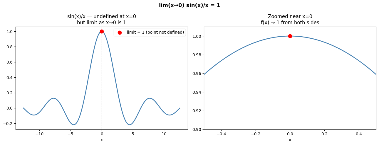
# Numerically verify: approach 0 from both sides
print('Approaching x=0 from the RIGHT:')
for x in [0.5, 0.1, 0.01, 0.001, 1e-6, 1e-10]:
    val = np.sin(x) / x
    print(f'  x = {x:.2e}   sin(x)/x = {val:.10f}')

print()
print('Approaching x=0 from the LEFT:')
for x in [-0.5, -0.1, -0.01, -0.001, -1e-6, -1e-10]:
    val = np.sin(x) / x
    print(f'  x = {x:.2e}   sin(x)/x = {val:.10f}')

print()
print('Both sides converge to 1.0 — the limit exists.')
Approaching x=0 from the RIGHT:
x = 5.00e-01 sin(x)/x = 0.9588510772
x = 1.00e-01 sin(x)/x = 0.9983341665
x = 1.00e-02 sin(x)/x = 0.9999833334
x = 1.00e-03 sin(x)/x = 0.9999998333
x = 1.00e-06 sin(x)/x = 1.0000000000
x = 1.00e-10 sin(x)/x = 1.0000000000
Approaching x=0 from the LEFT:
x = -5.00e-01 sin(x)/x = 0.9588510772
x = -1.00e-01 sin(x)/x = 0.9983341665
x = -1.00e-02 sin(x)/x = 0.9999833334
x = -1.00e-03 sin(x)/x = 0.9999998333
x = -1.00e-06 sin(x)/x = 1.0000000000
x = -1.00e-10 sin(x)/x = 1.0000000000
Both sides converge to 1.0 — the limit exists.
2. When Limits Don’t Exist
A limit fails to exist in three ways:
Left and right limits are different (jump discontinuity)
The function oscillates infinitely fast
The function goes to ±∞
fig, axes = plt.subplots(1, 3, figsize=(14, 4))

# 1. Jump discontinuity: Heaviside step function
x = np.linspace(-2, 2, 500)
step = np.where(x < 0, 0.0, 1.0)
axes[0].plot(x[x < 0],  step[x < 0],  color='steelblue', linewidth=2)
axes[0].plot(x[x >= 0], step[x >= 0], color='steelblue', linewidth=2)
axes[0].scatter([0], [0], color='steelblue', s=50, zorder=6, facecolors='white', edgecolors='steelblue', linewidths=2)
axes[0].scatter([0], [1], color='steelblue', s=50, zorder=6)
axes[0].set_title('Jump discontinuity\nlim(x→0) does not exist\n(left≠right)')
axes[0].axvline(0, color='red', linestyle='--', alpha=0.5)

# 2. Oscillation: sin(1/x)
x2_left  = np.linspace(-0.3, -1e-4, 5000)
x2_right = np.linspace( 1e-4,  0.3, 5000)
axes[1].plot(x2_left,  np.sin(1/x2_left),  color='steelblue', linewidth=0.8)
axes[1].plot(x2_right, np.sin(1/x2_right), color='steelblue', linewidth=0.8)
axes[1].set_title('Infinite oscillation\nlim(x→0) sin(1/x) does not exist')
axes[1].axvline(0, color='red', linestyle='--', alpha=0.5)

# 3. Divergence: 1/x^2
x3_left  = np.linspace(-2, -0.05, 300)
x3_right = np.linspace( 0.05,  2, 300)
axes[2].plot(x3_left,  1/x3_left**2,  color='steelblue', linewidth=2)
axes[2].plot(x3_right, 1/x3_right**2, color='steelblue', linewidth=2)
axes[2].set_ylim(0, 50)
axes[2].set_title('Divergence to ∞\nlim(x→0) 1/x² = ∞\n(limit is infinite)')
axes[2].axvline(0, color='red', linestyle='--', alpha=0.5)

plt.suptitle('Three Ways a Limit Can Fail to Exist', fontsize=13, fontweight='bold')
plt.tight_layout()
plt.show()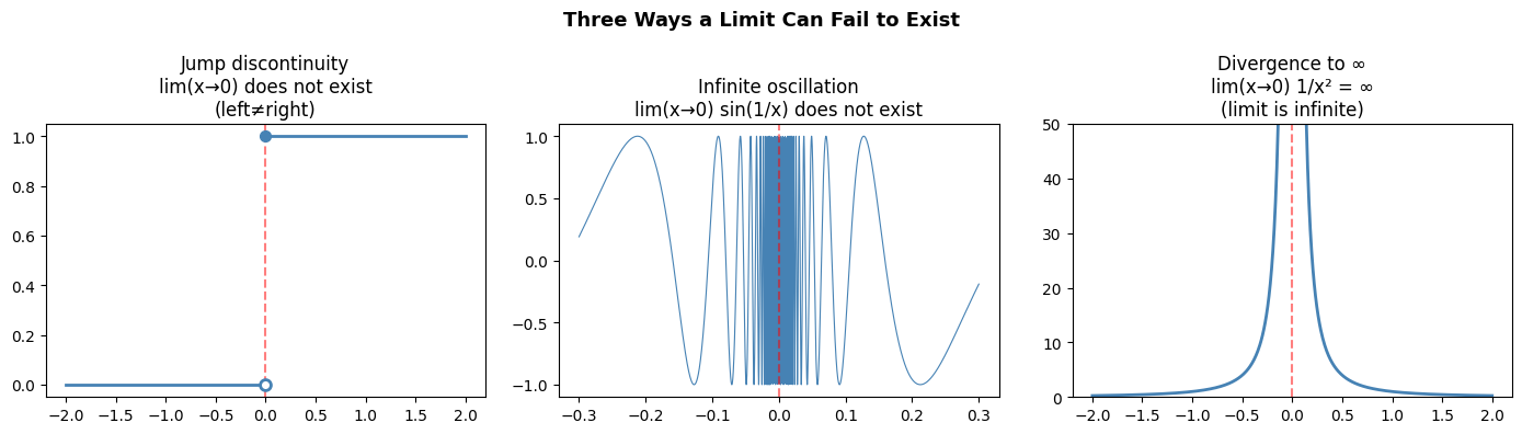
3. Limits at Infinity
We also care about behavior as x → ∞: what does a function approach as the input grows without bound?
x = np.linspace(1, 100, 500)

examples = {
    r'$1/x \to 0$':      lambda x: 1/x,
    r'$(x+1)/x \to 1$':  lambda x: (x+1)/x,
    r'$e^{-x} \to 0$':   lambda x: np.exp(-x),
    r'$\tanh(x) \to 1$': lambda x: np.tanh(x),
}

fig, ax = plt.subplots(figsize=(10, 5))
for label, fn in examples.items():
    ax.plot(x, fn(x), linewidth=2, label=label)

ax.set_xlabel('x')
ax.set_title('Limits as x → ∞')
ax.legend(fontsize=11)
ax.axhline(0, color='gray', linewidth=0.8)
ax.axhline(1, color='gray', linewidth=0.8, linestyle='--')
plt.tight_layout()
plt.show()

# Sigmoid-like functions approaching 1 are common in ML (activation functions)
# introduced in ch065 — Sigmoid Functions
print('tanh(100) =', np.tanh(100.0))
print('This is why tanh is called a "saturating" activation — it asymptotes to ±1.')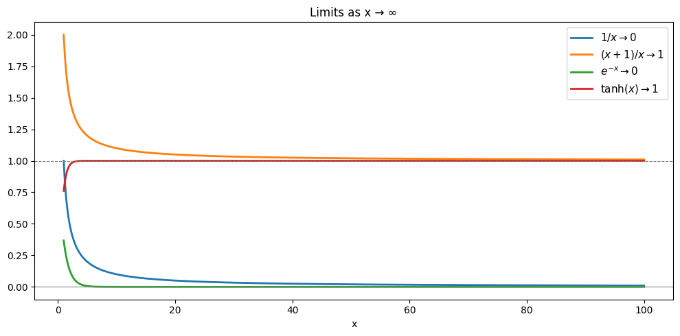
tanh(100) = 1.0
This is why tanh is called a "saturating" activation — it asymptotes to ±1.
4. The Limit as the Foundation of Derivatives
The definition of the derivative uses a limit directly:
Understanding limits means understanding why this formula makes sense: we’re computing the secant slope and asking what it approaches as the interval collapses. (Formalized in ch205 — Derivative Concept.)
5. Summary
A limit describes what a function approaches, not what it equals
Both the left limit and right limit must agree for a limit to exist
Limits at infinity describe long-run behavior (asymptotes)
The derivative is formally defined as a limit of a difference quotient
6. Forward References
The limit definition of the derivative is the subject of ch205 — Derivative Concept. Limits at infinity reappear in ch219 — Taylor Series, where the series approximation is valid in a neighborhood — and in ch241 — Randomness (Part VIII), where probability mass functions must sum to 1 in the limit.