Advanced Calculus Experiment 2.
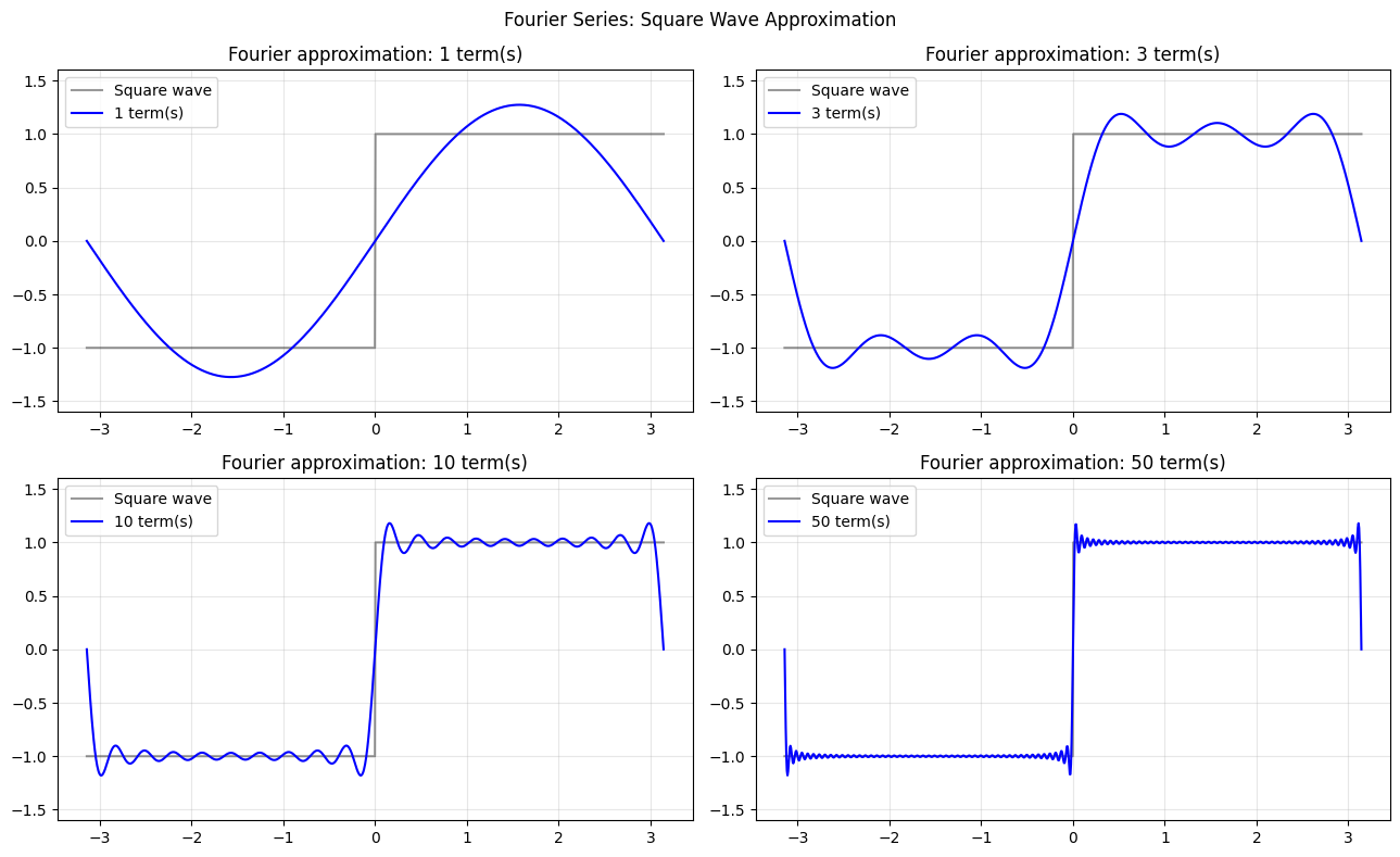
Any periodic function can be decomposed into an infinite sum of sines and cosines. This is the Fourier series. It is one of the most powerful ideas in applied mathematics — signal processing, audio compression, solving PDEs, and even neural network theory all rest on it.
import numpy as np
import matplotlib.pyplot as plt

# Fourier series of a square wave
# f(x) = (4/pi) * sum_{k=0}^{inf} sin((2k+1)x) / (2k+1)

x = np.linspace(-np.pi, np.pi, 1000)

def square_wave(x): return np.sign(np.sin(x))

def fourier_approx(x, n_terms):
    result = np.zeros_like(x, dtype=float)
    for k in range(n_terms):
        result += np.sin((2*k+1)*x) / (2*k+1)
    return 4/np.pi * result

fig, axes = plt.subplots(2, 2, figsize=(13, 8))
exact = square_wave(x)
for ax, n in zip(axes.flat, [1, 3, 10, 50]):
    ax.plot(x, exact, 'k', lw=1.5, alpha=0.4, label='Square wave')
    ax.plot(x, fourier_approx(x, n), 'b', lw=1.5, label=f'{n} term(s)')
    ax.set_ylim(-1.6, 1.6); ax.legend(); ax.grid(True, alpha=0.3)
    ax.set_title(f'Fourier approximation: {n} term(s)')
plt.suptitle('Fourier Series: Square Wave Approximation', fontsize=12)
plt.tight_layout(); plt.savefig('ch232_fourier_series.png', dpi=100); plt.show()
Fourier Coefficients
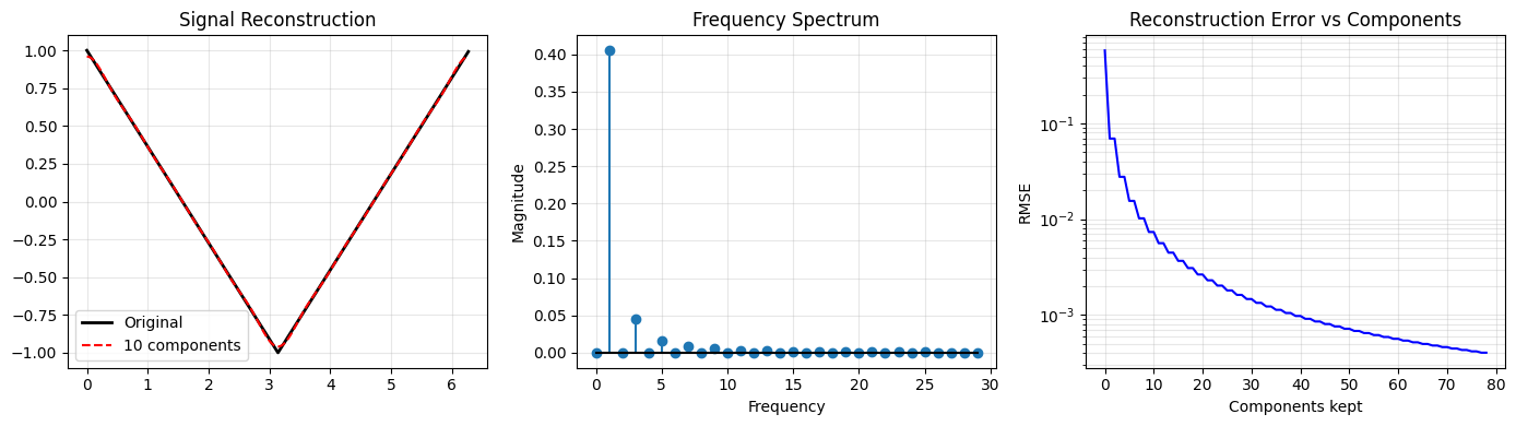
For a function f(x) with period 2pi, the Fourier coefficients are inner products:
a_k = (1/pi) * integral f(x) cos(kx) dx
b_k = (1/pi) * integral f(x) sin(kx) dx
Computing these numerically via the Discrete Fourier Transform (DFT) is the key operation in audio, image, and signal processing.
# Compute Fourier coefficients numerically and reconstruct
# Signal: triangular wave
N = 512
t = np.linspace(0, 2*np.pi, N, endpoint=False)
signal = 2*np.abs(t/np.pi - 1) - 1   # triangular wave in [-1,1]

# DFT (numpy's FFT)
freq_domain = np.fft.rfft(signal)
magnitudes = np.abs(freq_domain) / N

freqs = np.fft.rfftfreq(N, d=1/N)

# Reconstruct from only first 10 Fourier components
freq_truncated = np.zeros_like(freq_domain)
freq_truncated[:10] = freq_domain[:10]
reconstructed = np.fft.irfft(freq_truncated, n=N)

fig, axes = plt.subplots(1, 3, figsize=(14, 4))
axes[0].plot(t, signal, 'k', lw=2, label='Original')
axes[0].plot(t, reconstructed, 'r--', lw=1.5, label='10 components')
axes[0].legend(); axes[0].set_title('Signal Reconstruction'); axes[0].grid(True, alpha=0.3)

axes[1].stem(freqs[:30], magnitudes[:30], markerfmt='C0o', linefmt='C0-', basefmt='k-')
axes[1].set_xlabel('Frequency'); axes[1].set_ylabel('Magnitude')
axes[1].set_title('Frequency Spectrum'); axes[1].grid(True, alpha=0.3)

# Reconstruction error vs number of components
errs = []
for k in range(1, 80):
    ft = np.zeros_like(freq_domain); ft[:k] = freq_domain[:k]
    rec = np.fft.irfft(ft, n=N)
    errs.append(np.sqrt(np.mean((rec - signal)**2)))
axes[2].semilogy(errs, 'b-'); axes[2].set_xlabel('Components kept')
axes[2].set_ylabel('RMSE'); axes[2].set_title('Reconstruction Error vs Components')
axes[2].grid(True, which='both', alpha=0.3)
plt.tight_layout(); plt.savefig('ch232_fft.png', dpi=100); plt.show()
Summary
| Concept | Key Idea |
|---|---|
| Fourier series | Decompose periodic f into sin/cos components |
| Fourier coefficients | Inner products with basis functions |
| DFT / FFT | Discrete version; O(N log N) algorithm |
| Gibbs phenomenon | Ringing near discontinuities — never fully disappears |
Forward reference: ch298 — Information Theory (Part IX) builds on frequency-domain ideas to define entropy and information content.