Part VIII: Probability | Computational Mathematics for Programmers
1. Spread Around the Mean
Expected value (ch249) tells you where the distribution is centered. It tells you nothing about how spread out it is. Two distributions can have the same mean but radically different spread.
Variance measures the expected squared deviation from the mean:
where μ = E[X].
Standard deviation: σ = √Var(X). Same units as X, which makes it interpretable.
import numpy as np
import matplotlib.pyplot as plt
from scipy import stats

# Two distributions with same mean but different variance
mu = 5

x = np.linspace(0, 10, 500)
rv_narrow = stats.norm(loc=mu, scale=0.5)
rv_wide   = stats.norm(loc=mu, scale=2.0)

fig, ax = plt.subplots(figsize=(8, 4))
ax.plot(x, rv_narrow.pdf(x), 'steelblue', linewidth=2, label='μ=5, σ=0.5 (low variance)')
ax.plot(x, rv_wide.pdf(x),   'tomato',    linewidth=2, label='μ=5, σ=2.0 (high variance)')
ax.axvline(mu, color='black', linestyle='--', alpha=0.5, label='Mean = 5')
ax.set_xlabel('x')
ax.set_ylabel('f(x)')
ax.set_title('Same Mean, Different Variance')
ax.legend()
plt.tight_layout()
plt.show()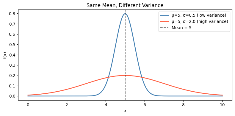
def variance_discrete(values, probs):
    values, probs = np.array(values, float), np.array(probs, float)
    mu = np.sum(values * probs)
    # Definition: E[(X-mu)^2]
    var_def = np.sum((values - mu)**2 * probs)
    # Computational: E[X^2] - mu^2
    var_comp = np.sum(values**2 * probs) - mu**2
    return mu, var_def, var_comp

faces = np.arange(1, 7)
pmf = np.full(6, 1/6)

mu, var_def, var_comp = variance_discrete(faces, pmf)
print(f"Fair die:")
print(f"  μ = E[X] = {mu:.4f}")
print(f"  Var(X) via definition = {var_def:.6f}")
print(f"  Var(X) via E[X²]-μ²  = {var_comp:.6f}")
print(f"  σ = √Var(X) = {np.sqrt(var_def):.4f}")
print(f"  numpy agrees: {np.isclose(var_def, np.var([1,2,3,4,5,6]))}")  # ddof=0 (population)
Fair die:
μ = E[X] = 3.5000
Var(X) via definition = 2.916667
Var(X) via E[X²]-μ² = 2.916667
σ = √Var(X) = 1.7078
numpy agrees: True
3. Variance of Scaled and Shifted Variables
Note: adding a constant b shifts the distribution but does not change its spread. Scaling by a multiplies the variance by a².
This is why standard deviation scales linearly with the variable (σ(aX) = |a|σ) while variance scales quadratically.
# Verify Var(aX + b) = a^2 * Var(X)
a, b = 3, 10

mu_X, var_X, _ = variance_discrete(faces, pmf)

# Y = aX + b
y_values = a * faces + b
mu_Y, var_Y, _ = variance_discrete(y_values, pmf)

print(f"X: μ={mu_X:.4f}, Var={var_X:.4f}")
print(f"Y = {a}X + {b}: μ={mu_Y:.4f}, Var={var_Y:.4f}")
print(f"Expected Var(Y) = a²·Var(X) = {a}²×{var_X:.4f} = {a**2 * var_X:.4f}")
print(f"Match: {np.isclose(var_Y, a**2 * var_X)}")
X: μ=3.5000, Var=2.9167
Y = 3X + 10: μ=20.5000, Var=26.2500
Expected Var(Y) = a²·Var(X) = 3²×2.9167 = 26.2500
Match: True
4. Variance of Sums (Independent RVs)
For independent random variables X and Y:
For dependent variables, you need the covariance:
from itertools import product

# Var(die1 + die2) should equal Var(die1) + Var(die2)
Omega2 = list(product(faces, faces))
p2 = 1 / len(Omega2)

sums = np.array([d1 + d2 for d1, d2 in Omega2])
E_sum = sums.mean()
Var_sum = np.mean((sums - E_sum)**2)

print(f"Var(die1 + die2) = {Var_sum:.4f}")
print(f"Var(die1) + Var(die2) = {var_X + var_X:.4f}")
print(f"Match: {np.isclose(Var_sum, 2 * var_X)}")

# Standard deviation scales as sqrt(n) for n independent identically-distributed vars
print("\nσ scaling for n independent dice:")
sigma_one = np.sqrt(var_X)
for n in [1, 4, 9, 25, 100]:
    sigma_sum = np.sqrt(n) * sigma_one
    print(f"  n={n:3d}: σ(sum) = √{n}×{sigma_one:.4f} = {sigma_sum:.4f}")
Var(die1 + die2) = 5.8333
Var(die1) + Var(die2) = 5.8333
Match: True
σ scaling for n independent dice:
n= 1: σ(sum) = √1×1.7078 = 1.7078
n= 4: σ(sum) = √4×1.7078 = 3.4157
n= 9: σ(sum) = √9×1.7078 = 5.1235
n= 25: σ(sum) = √25×1.7078 = 8.5391
n=100: σ(sum) = √100×1.7078 = 17.0783
5. Sample Variance vs Population Variance
From a sample of n observations, the biased estimator divides by n; the unbiased estimator divides by n−1 (Bessel’s correction):
# Demonstrate why n-1 not n for sample variance
rng = np.random.default_rng(seed=42)
true_variance = var_X  # known for fair die

n_simulations = 10_000
sample_size = 10

biased_estimates = []
unbiased_estimates = []

for _ in range(n_simulations):
    sample = rng.choice(faces, size=sample_size, p=pmf)
    biased_estimates.append(np.var(sample, ddof=0))    # divide by n
    unbiased_estimates.append(np.var(sample, ddof=1))  # divide by n-1

print(f"True population variance: {true_variance:.4f}")
print(f"Average biased estimate (ddof=0):   {np.mean(biased_estimates):.4f}  <- underestimates")
print(f"Average unbiased estimate (ddof=1): {np.mean(unbiased_estimates):.4f}  <- matches")
print(f"\nUse ddof=1 when estimating variance from a sample.")
print(f"Use ddof=0 for the population (when you have all data).")
True population variance: 2.9167
Average biased estimate (ddof=0): 2.6197 <- underestimates
Average unbiased estimate (ddof=1): 2.9108 <- matches
Use ddof=1 when estimating variance from a sample.
Use ddof=0 for the population (when you have all data).
6. Summary
Var(X) = E[(X−μ)²] = E[X²] − E[X]² measures spread around the mean.
σ = √Var(X) is the standard deviation — same units as X.
Var(aX+b) = a²·Var(X): constants shift the mean, not the spread; scaling multiplies variance by a².
For independent RVs: Var(X+Y) = Var(X) + Var(Y). Dependent variables require covariance terms.
Sample variance divides by n−1 (unbiased); population variance divides by n.
7. Forward References
Mean and variance are the first two moments of a distribution. They appear in the normal distribution (ch253) as its defining parameters. The Central Limit Theorem (ch254) states that sums of random variables with finite mean and variance converge to a normal distribution — this is why σ/√n appears in confidence intervals (Part IX, ch280). Covariance generalizes variance to pairs of variables and becomes the covariance matrix in Part VI linear algebra (introduced in ch176) and Part IX regression (ch281).