Part VIII: Probability | Computational Mathematics for Programmers
1. The Setup: n Independent Binary Trials
You have n independent experiments, each with probability p of “success” and (1−p) of “failure”. How many successes do you get?
This is the binomial distribution: X ~ Binomial(n, p).
Examples:
Flip 10 coins. How many heads? X ~ Binomial(10, 0.5)
Test 100 users. How many convert? X ~ Binomial(100, 0.03)
Read 8 bits. How many are flipped by noise? X ~ Binomial(8, 0.01)
2. Derivation of the PMF
P(exactly k successes in n trials):
The probability of any specific arrangement with k successes and (n−k) failures is p^k · (1−p)^(n−k) (independence).
The number of such arrangements is C(n,k) = n! / (k!(n−k)!) — the binomial coefficient.
import numpy as np
import matplotlib.pyplot as plt
from scipy import stats
from math import comb

def binomial_pmf(n, p, k):
    """P(X=k) for X ~ Binomial(n, p). Implemented from scratch."""
    return comb(n, k) * (p ** k) * ((1 - p) ** (n - k))


# Verify against scipy
n, p = 10, 0.3
for k in range(n + 1):
    ours = binomial_pmf(n, p, k)
    scipy_val = stats.binom.pmf(k, n, p)
    match = np.isclose(ours, scipy_val)
    print(f"P(X={k:2d}) = {ours:.6f}  scipy={scipy_val:.6f}  match={match}")
P(X= 0) = 0.028248 scipy=0.028248 match=True
P(X= 1) = 0.121061 scipy=0.121061 match=True
P(X= 2) = 0.233474 scipy=0.233474 match=True
P(X= 3) = 0.266828 scipy=0.266828 match=True
P(X= 4) = 0.200121 scipy=0.200121 match=True
P(X= 5) = 0.102919 scipy=0.102919 match=True
P(X= 6) = 0.036757 scipy=0.036757 match=True
P(X= 7) = 0.009002 scipy=0.009002 match=True
P(X= 8) = 0.001447 scipy=0.001447 match=True
P(X= 9) = 0.000138 scipy=0.000138 match=True
P(X=10) = 0.000006 scipy=0.000006 match=True
# Visualize for different parameters
fig, axes = plt.subplots(2, 2, figsize=(11, 8))
configs = [
    (10, 0.5, 'Binomial(10, 0.5)'),
    (10, 0.2, 'Binomial(10, 0.2)'),
    (50, 0.3, 'Binomial(50, 0.3)'),
    (100, 0.05, 'Binomial(100, 0.05)'),
]

for ax, (n, p, title) in zip(axes.flat, configs):
    k = np.arange(0, n + 1)
    pmf = stats.binom.pmf(k, n, p)
    mu = n * p
    sigma = np.sqrt(n * p * (1 - p))

    ax.bar(k, pmf, color='steelblue', alpha=0.8, edgecolor='white')
    ax.axvline(mu, color='tomato', linestyle='--', label=f'μ={mu:.1f}')
    ax.set_title(title)
    ax.set_xlabel('k')
    ax.set_ylabel('P(X=k)')
    ax.legend(fontsize=9)

plt.tight_layout()
plt.show()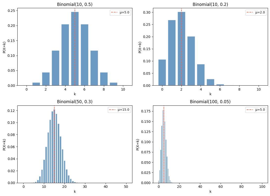
3. Mean and Variance
For X ~ Binomial(n, p):
Proof via linearity of expectation: X = X₁ + X₂ + ... + Xₙ where each Xᵢ ~ Bernoulli(p). E[Xᵢ] = p, Var(Xᵢ) = p(1−p). By linearity and independence: E[X] = np, Var(X) = np(1−p).
def binomial_stats(n, p):
    mu = n * p
    var = n * p * (1 - p)
    return mu, var

configs = [(10, 0.5), (50, 0.3), (100, 0.05)]
print(f"{'n':>6} {'p':>6} {'E[X]=np':>12} {'Var=np(1-p)':>14} {'σ':>8}")
print("-" * 50)
for n, p in configs:
    mu, var = binomial_stats(n, p)
    # Verify with scipy
    rv = stats.binom(n, p)
    assert np.isclose(rv.mean(), mu) and np.isclose(rv.var(), var)
    print(f"{n:>6} {p:>6.2f} {mu:>12.4f} {var:>14.4f} {np.sqrt(var):>8.4f}")
n p E[X]=np Var=np(1-p) σ
--------------------------------------------------
10 0.50 5.0000 2.5000 1.5811
50 0.30 15.0000 10.5000 3.2404
100 0.05 5.0000 4.7500 2.1794
4. Applications
A/B Testing
You run an experiment: 200 users see variant A, 200 see variant B. Variant A has 24 conversions, variant B has 34. Is B actually better, or is this variance?
# Under H₀: both have p=0.14 (pooled rate)
n_A, k_A = 200, 24
n_B, k_B = 200, 34

p_A = k_A / n_A
p_B = k_B / n_B
p_pool = (k_A + k_B) / (n_A + n_B)

print(f"Conversion rate A: {p_A:.4f}")
print(f"Conversion rate B: {p_B:.4f}")
print(f"Pooled rate: {p_pool:.4f}")

# P(getting >= 34 conversions under H₀) — one-sided
# Under H₀, k_B ~ Binomial(200, p_pool)
p_value = 1 - stats.binom.cdf(k_B - 1, n_B, p_pool)
print(f"\nP(X >= {k_B} | p={p_pool:.4f}) = {p_value:.4f}")
print(f"Conclusion: {'Significant at α=0.05' if p_value < 0.05 else 'Not significant at α=0.05'}")
Conversion rate A: 0.1200
Conversion rate B: 0.1700
Pooled rate: 0.1450
P(X >= 34 | p=0.1450) = 0.1818
Conclusion: Not significant at α=0.05
5. Binomial → Normal Approximation
For large n, Binomial(n, p) is well-approximated by Normal(np, np(1−p)). This is an instance of the Central Limit Theorem (ch254).
n, p = 200, 0.14
mu, var = n * p, n * p * (1 - p)
sigma = np.sqrt(var)

k = np.arange(0, n + 1)
binom_pmf = stats.binom.pmf(k, n, p)

x_norm = np.linspace(mu - 4*sigma, mu + 4*sigma, 300)
norm_pdf = stats.norm.pdf(x_norm, mu, sigma)

fig, ax = plt.subplots(figsize=(8, 4))
ax.bar(k, binom_pmf, color='steelblue', alpha=0.7, label=f'Binomial({n},{p})')
ax.plot(x_norm, norm_pdf, 'tomato', linewidth=2, label=f'Normal(μ={mu:.1f}, σ={sigma:.2f})')
ax.set_xlim(mu - 4*sigma, mu + 4*sigma)
ax.set_xlabel('k')
ax.set_ylabel('Probability')
ax.set_title('Binomial approximated by Normal (large n)')
ax.legend()
plt.tight_layout()
plt.show()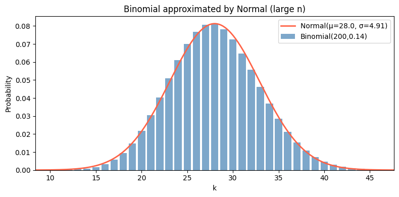
6. Summary
X ~ Binomial(n, p): count of successes in n independent Bernoulli(p) trials.
PMF: P(X=k) = C(n,k) · p^k · (1−p)^(n−k).
E[X] = np, Var(X) = np(1−p) — derived via linearity from Bernoulli components.
For large n: approximates Normal(np, np(1−p)) by the Central Limit Theorem.
7. Forward References
The Poisson distribution (ch252) is the limit of Binomial(n, p) as n→∞ and p→0 with np=λ fixed. It models rare events in large trials. The normal approximation to the binomial is the simplest case of the Central Limit Theorem (ch254), which generalizes it to sums of any independent random variables.