Chapter 258 — Random Walks - Mathematics for Programmers

Part VIII: Probability¶

A random walk is the trajectory of a particle that at each step moves by a random displacement. The simplest version — the 1D symmetric random walk — is the gateway to Brownian motion, the diffusion equation, option pricing, polymer physics, and network theory.

What makes random walks special is that despite being defined by i.i.d. increments, they produce correlated trajectories. The position at time $n$ depends on all previous positions. Yet this correlation has a precise mathematical structure we can analyze exactly.

Prerequisites: Random Variables (ch247), Variance and Standard Deviation (ch250), Markov Chains (ch257), Central Limit Theorem (ch254).

1. The 1D Symmetric Random Walk¶

Let $X_1, X_2, \ldots$ be i.i.d. with $P(X_i = +1) = P(X_i = -1) = 1/2$ . Define:

S_n = \sum_{k=1}^n X_k, \quad S_0 = 0

(1)

Key exact results:

$\mathbb{E}[S_n] = 0$ (unbiased steps)
$\text{Var}(S_n) = n$ (variance grows linearly)
$\text{Std}(S_n) = \sqrt{n}$ (spread grows as square root)

The $\sqrt{n}$ growth is a fundamental signature of diffusion.

import numpy as np
import matplotlib.pyplot as plt
from scipy import stats

rng = np.random.default_rng(42)

def random_walk_1d(n_steps, n_walks, p=0.5, rng=None):
    """Simulate multiple 1D random walks.
    
    Args:
        n_steps: number of steps per walk
        n_walks: number of independent walks
        p: probability of step +1 (default 0.5 = symmetric)
        rng: numpy random generator
    
    Returns:
        positions: (n_steps+1, n_walks) array of positions
    """
    if rng is None:
        rng = np.random.default_rng()
    steps = rng.choice([-1, 1], size=(n_steps, n_walks), p=[1-p, p])
    positions = np.zeros((n_steps + 1, n_walks), dtype=int)
    positions[1:] = np.cumsum(steps, axis=0)
    return positions

n_steps = 500
n_walks = 200
walks = random_walk_1d(n_steps, n_walks, rng=rng)
t = np.arange(n_steps + 1)

fig, axes = plt.subplots(1, 2, figsize=(14, 5))

# Left: individual walks + spread envelope
for i in range(min(30, n_walks)):
    axes[0].plot(t, walks[:, i], alpha=0.15, linewidth=0.8, color='steelblue')
axes[0].plot(t, 2*np.sqrt(t), 'r--', linewidth=2, label='+2√t')
axes[0].plot(t, -2*np.sqrt(t), 'r--', linewidth=2, label='-2√t')
axes[0].set_xlabel('Step n')
axes[0].set_ylabel('Position S_n')
axes[0].set_title('30 Random Walks (symmetric, 1D)')
axes[0].legend()
axes[0].grid(True, alpha=0.3)

# Right: std(S_n) vs sqrt(n)
empirical_std = np.std(walks, axis=1)
axes[1].plot(t, empirical_std, 'b-', label='Empirical std(S_n)', linewidth=2)
axes[1].plot(t, np.sqrt(t), 'r--', label='√n (theoretical)', linewidth=2)
axes[1].set_xlabel('Step n')
axes[1].set_ylabel('Standard Deviation')
axes[1].set_title('Growth of Spread: √n Law')
axes[1].legend()
axes[1].grid(True, alpha=0.3)

plt.tight_layout()
plt.savefig('random_walk_1d.png', dpi=120, bbox_inches='tight')
plt.show()

print(f"At n={n_steps}: empirical std = {empirical_std[-1]:.2f}, √n = {np.sqrt(n_steps):.2f}")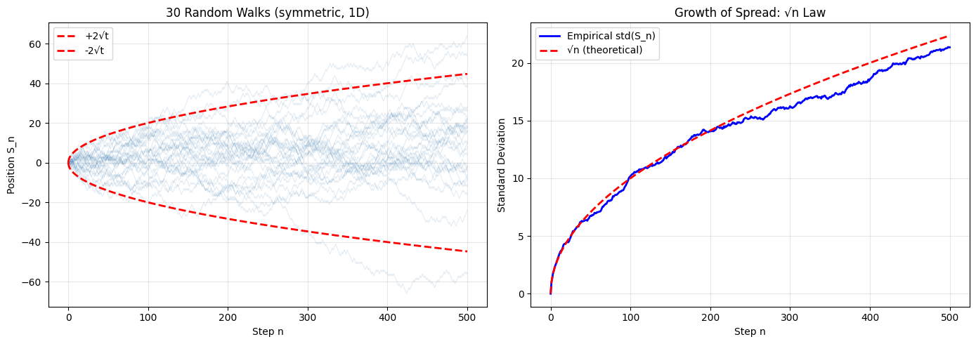

At n=500: empirical std = 21.35, √n = 22.36

2. The CLT View: Brownian Motion in the Limit¶

By the CLT (ch254), $S_n / \sqrt{n} \to N(0,1)$ as $n \to \infty$ . More precisely:

\frac{S_{\lfloor nt \rfloor}}{\sqrt{n}} \xrightarrow{d} B(t)

(2)

where $B(t)$ is Brownian motion (Wiener process). This is Donsker’s theorem. The random walk is the discrete skeleton of Brownian motion.

# Verify distribution of S_n is approximately Normal
ns_to_check = [10, 50, 200]

fig, axes = plt.subplots(1, 3, figsize=(15, 4))
for ax, n in zip(axes, ns_to_check):
    positions_at_n = walks[n, :]
    
    # Histogram
    ax.hist(positions_at_n / np.sqrt(n), bins=25, density=True,
            color='steelblue', alpha=0.7, edgecolor='white')
    
    # Overlay N(0,1)
    x_range = np.linspace(-4, 4, 200)
    ax.plot(x_range, stats.norm.pdf(x_range), 'r-', linewidth=2, label='N(0,1)')
    
    # QQ test
    ks_stat, ks_p = stats.kstest(positions_at_n / np.sqrt(n), 'norm')
    ax.set_title(f'n={n}\nKS p-value: {ks_p:.3f}')
    ax.set_xlabel(f'S_{n} / √{n}')
    ax.set_ylabel('Density')
    ax.legend()
    ax.grid(True, alpha=0.3)

plt.suptitle('Distribution of S_n/√n converges to N(0,1)', y=1.02)
plt.tight_layout()
plt.savefig('random_walk_clt.png', dpi=120, bbox_inches='tight')
plt.show()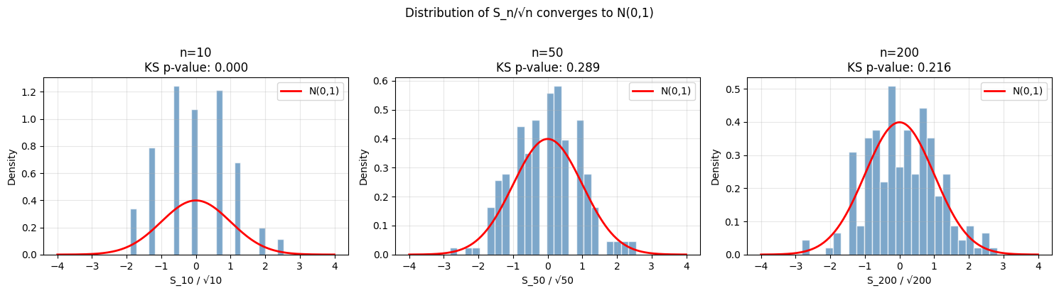

3. First Passage Times and the Gambler’s Ruin¶

How long does the walk take to first reach level $a > 0$ ? This is the first passage time $T_a = \min\{n : S_n = a\}$ .

Gambler’s Ruin: A gambler starts with $k$ dollars, plays against a casino with infinite funds, winning $1 with probability$ p $and losing$ 1 with probability $q = 1-p$ . The probability of ruin (reaching 0) is:

P(\text{ruin} \mid S_0 = k) = \begin{cases} \left(\frac{q}{p}\right)^k & p \neq 1/2 \\ 1 & p = 1/2 \end{cases}

(3)

At $p = 1/2$ , the symmetric walk is recurrent — it returns to every point infinitely often, and ruin is certain.

def gambler_ruin_simulation(k, target, p, n_trials, max_steps=50_000, rng=None):
    """Simulate Gambler's Ruin.
    
    Args:
        k: starting wealth
        target: winning target (reach this = win)
        p: probability of winning each bet
        n_trials: number of independent games to simulate
        max_steps: truncation (treat as draw if exceeded)
        rng: numpy random generator
    
    Returns:
        ruin_rate: fraction of games ending in ruin
        win_rate: fraction of games where target was reached
        mean_duration: mean game length (of completed games)
    """
    if rng is None:
        rng = np.random.default_rng()
    
    ruin_count = 0
    win_count = 0
    durations = []
    
    for _ in range(n_trials):
        wealth = k
        steps = 0
        while 0 < wealth < target and steps < max_steps:
            if rng.random() < p:
                wealth += 1
            else:
                wealth -= 1
            steps += 1
        
        if wealth == 0:
            ruin_count += 1
            durations.append(steps)
        elif wealth == target:
            win_count += 1
            durations.append(steps)
    
    return ruin_count/n_trials, win_count/n_trials, np.mean(durations) if durations else np.nan

# Compare fair vs biased games
k = 10  # starting wealth
target = 20  # win target
n_trials = 2000

print(f"Gambler's Ruin: start={k}, target={target}")
print(f"{'p':>6} {'Ruin prob (sim)':>16} {'Ruin prob (theory)':>20} {'Mean duration':>14}")
print("-" * 62)

for p in [0.4, 0.45, 0.5, 0.55, 0.6]:
    ruin_rate, win_rate, mean_dur = gambler_ruin_simulation(k, target, p, n_trials, rng=rng)
    
    q = 1 - p
    if abs(p - 0.5) < 1e-9:
        theory_ruin = 1 - k/target  # fair game: P(ruin|start k, target N) = 1 - k/N
    else:
        r = q/p
        theory_ruin = (r**k - r**target) / (1 - r**target)  # biased: Feller formula
    
    print(f"{p:>6.2f} {ruin_rate:>16.4f} {theory_ruin:>20.4f} {mean_dur:>14.1f}")

Gambler's Ruin: start=10, target=20
     p  Ruin prob (sim)   Ruin prob (theory)  Mean duration
--------------------------------------------------------------
  0.40           0.9810               0.9830           48.8
  0.45           0.8745               0.8815           75.6
  0.50           0.4820               0.5000           99.5
  0.55           0.1215               0.1185           76.5
  0.60           0.0155               0.0170           49.2

4. 2D Random Walks¶

In 2D, the walker moves N/S/E/W at each step. Key result: the 2D walk is also recurrent (returns to origin with probability 1). In 3D or higher, walks are transient — they escape to infinity. This is Pólya’s theorem (1921).

def random_walk_2d(n_steps, rng):
    """2D random walk on integer lattice (N/S/E/W)."""
    directions = np.array([[0,1],[0,-1],[1,0],[-1,0]])
    choices = rng.integers(0, 4, size=n_steps)
    steps = directions[choices]
    positions = np.zeros((n_steps + 1, 2), dtype=int)
    positions[1:] = np.cumsum(steps, axis=0)
    return positions

n_steps = 5000
walk_2d = random_walk_2d(n_steps, rng)

fig, axes = plt.subplots(1, 2, figsize=(14, 5))

# Trajectory
sc = axes[0].scatter(walk_2d[:, 0], walk_2d[:, 1],
                     c=np.arange(n_steps+1), cmap='viridis',
                     s=0.5, alpha=0.7)
axes[0].plot(*walk_2d[0], 'go', markersize=10, label='Start', zorder=5)
axes[0].plot(*walk_2d[-1], 'r*', markersize=12, label='End', zorder=5)
plt.colorbar(sc, ax=axes[0], label='Step')
axes[0].set_title(f'2D Random Walk ({n_steps} steps)')
axes[0].set_xlabel('x')
axes[0].set_ylabel('y')
axes[0].legend()
axes[0].grid(True, alpha=0.3)
axes[0].set_aspect('equal')

# Distance from origin over time
t = np.arange(n_steps + 1)
dist = np.sqrt(walk_2d[:, 0]**2 + walk_2d[:, 1]**2)
axes[1].plot(t, dist, 'b-', alpha=0.6, linewidth=0.8, label='|S_n|')
axes[1].plot(t, np.sqrt(2 * t), 'r--', linewidth=2, label='√(2n) (theoretical mean)')
axes[1].set_xlabel('Step n')
axes[1].set_ylabel('Distance from origin')
axes[1].set_title('Distance from Origin vs √(2n)')
axes[1].legend()
axes[1].grid(True, alpha=0.3)

plt.tight_layout()
plt.savefig('random_walk_2d.png', dpi=120, bbox_inches='tight')
plt.show()

final_dist = dist[-1]
theoretical_mean = np.sqrt(2 * n_steps)
print(f"Final distance: {final_dist:.1f}")
print(f"Theoretical E[|S_n|] ≈ √(2n) = {theoretical_mean:.1f}")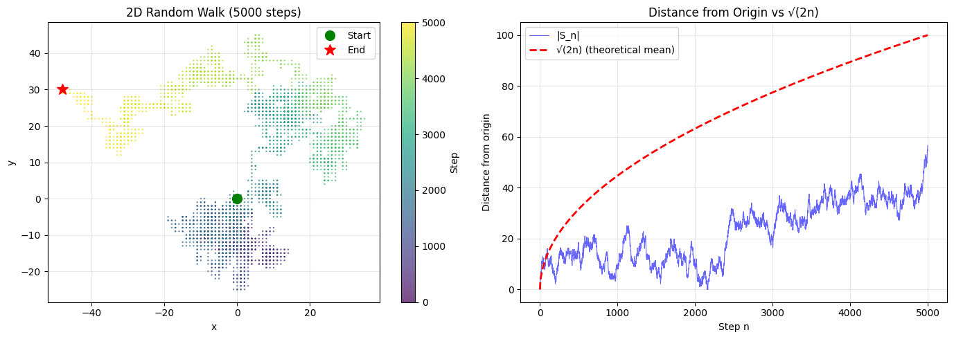

Final distance: 56.6
Theoretical E[|S_n|] ≈ √(2n) = 100.0

5. Self-Avoiding Walks and Applications¶

A self-avoiding walk (SAW) must not revisit any site. SAWs model polymer chains in statistical physics — each monomer occupies a distinct location in space. Unlike simple random walks, SAWs are non-Markovian (future steps depend on all past positions).

def self_avoiding_walk(max_steps, rng, max_attempts=10000):
    """Generate a self-avoiding walk using backtracking (pivot-free version).
    Uses repeated attempts (not full backtracking) for simplicity.
    Returns the longest walk found within max_attempts tries.
    """
    directions = [(0,1),(0,-1),(1,0),(-1,0)]
    best_walk = [(0, 0)]
    
    for _ in range(max_attempts):
        visited = {(0, 0)}
        path = [(0, 0)]
        pos = (0, 0)
        
        for _ in range(max_steps):
            shuffled = rng.permutation(len(directions))
            moved = False
            for di in shuffled:
                dx, dy = directions[di]
                new_pos = (pos[0] + dx, pos[1] + dy)
                if new_pos not in visited:
                    visited.add(new_pos)
                    path.append(new_pos)
                    pos = new_pos
                    moved = True
                    break
            if not moved:  # trapped
                break
        
        if len(path) > len(best_walk):
            best_walk = path
    
    return best_walk

saw = self_avoiding_walk(max_steps=200, rng=rng, max_attempts=500)
saw_arr = np.array(saw)

fig, ax = plt.subplots(figsize=(7, 7))
n_pts = len(saw_arr)
sc = ax.scatter(saw_arr[:, 0], saw_arr[:, 1],
                c=np.arange(n_pts), cmap='plasma', s=15, zorder=3)
ax.plot(saw_arr[:, 0], saw_arr[:, 1], 'k-', alpha=0.3, linewidth=0.8)
ax.plot(*saw_arr[0], 'go', markersize=10, label='Start', zorder=5)
ax.plot(*saw_arr[-1], 'r*', markersize=12, label='End', zorder=5)
plt.colorbar(sc, ax=ax, label='Step')
ax.set_title(f'Self-Avoiding Walk ({n_pts-1} steps before trapped)')
ax.set_aspect('equal')
ax.legend()
ax.grid(True, alpha=0.3)
plt.tight_layout()
plt.savefig('self_avoiding_walk.png', dpi=120, bbox_inches='tight')
plt.show()

end_to_end = np.sqrt(((saw_arr[-1] - saw_arr[0])**2).sum())
print(f"Walk length: {n_pts-1} steps")
print(f"End-to-end distance: {end_to_end:.2f}")
print(f"(Simple RW would give ~√n = {np.sqrt(n_pts-1):.2f})")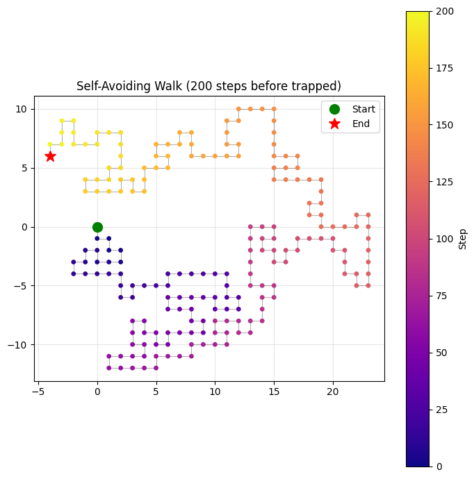

Walk length: 200 steps
End-to-end distance: 7.21
(Simple RW would give ~√n = 14.14)

6. Summary¶

Property	1D Symmetric RW	Result
Mean position	$\mathbb{E}[S_n] = 0$	Unbiased
Spread	$\text{Std}(S_n) = \sqrt{n}$	Diffusive scaling
Distribution	$S_n/\sqrt{n} \to N(0,1)$	CLT applies
Recurrence (1D, 2D)	Returns to origin w.p. 1	Pólya’s theorem
Transience (3D+)	Escapes to infinity	Pólya’s theorem
Gambler’s ruin (fair)	Ruin prob = $1 - k/N$	Always ruins eventually

9. Forward References¶

ch259 — Simulation Techniques: Builds general simulation infrastructure for SDEs (stochastic differential equations) — the continuous analog of random walks, used in finance (Black-Scholes) and physics.
ch279 — Correlation (Part IX): The autocovariance $\text{Cov}(S_m, S_n) = \min(m,n)$ captures how random walk positions are correlated — a direct application of covariance structure.