Chapter 264 — Stochastic Processes and Queuing Theory

import numpy as np
import matplotlib.pyplot as plt
from scipy import stats

rng = np.random.default_rng(42)

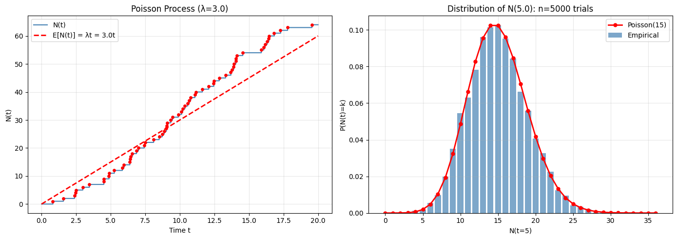
## 1. The Poisson Process
# Events arrive at rate lambda. Inter-arrival times ~ Exp(lambda).
# N(t) = number of arrivals by time t ~ Poisson(lambda * t)

def simulate_poisson_process(rate, t_max, rng):
    """Simulate a homogeneous Poisson process up to t_max.
    
    Args:
        rate: arrival rate lambda (events per unit time)
        t_max: simulation end time
        rng: numpy random generator
    
    Returns:
        arrival_times: array of arrival times in [0, t_max]
    """
    # Generate Exponential inter-arrivals until we exceed t_max
    arrivals = []
    t = 0.0
    while True:
        inter_arrival = rng.exponential(1.0 / rate)
        t += inter_arrival
        if t > t_max:
            break
        arrivals.append(t)
    return np.array(arrivals)

lam = 3.0  # 3 arrivals per unit time
t_max = 20.0

arrivals = simulate_poisson_process(lam, t_max, rng)
print(f"λ={lam}, T={t_max}: observed {len(arrivals)} arrivals")
print(f"Expected: {lam * t_max:.1f}, Std: {np.sqrt(lam * t_max):.2f}")

# Count process N(t)
t_grid = np.linspace(0, t_max, 1000)
N_t = np.array([np.sum(arrivals <= t) for t in t_grid])

fig, axes = plt.subplots(1, 2, figsize=(14, 5))

axes[0].step(t_grid, N_t, where='post', color='steelblue', linewidth=1.5, label='N(t)')
axes[0].plot(t_grid, lam * t_grid, 'r--', linewidth=2, label=f'E[N(t)] = λt = {lam}t')
axes[0].scatter(arrivals, np.arange(1, len(arrivals)+1), color='red', s=15, zorder=5)
axes[0].set_xlabel('Time t')
axes[0].set_ylabel('N(t)')
axes[0].set_title(f'Poisson Process (λ={lam})')
axes[0].legend()
axes[0].grid(True, alpha=0.3)

# Distribution of N(t=5): should be Poisson(lambda*5)
t_check = 5.0
n_trials = 5000
counts = [len(simulate_poisson_process(lam, t_check, rng)) for _ in range(n_trials)]
expected_lam = lam * t_check

k_vals = np.arange(0, int(expected_lam * 2.5))
axes[1].bar(k_vals, [np.mean(np.array(counts) == k) for k in k_vals],
            alpha=0.7, color='steelblue', label='Empirical')
axes[1].plot(k_vals, stats.poisson.pmf(k_vals, expected_lam), 'ro-',
             linewidth=2, markersize=5, label=f'Poisson({expected_lam:.0f})')
axes[1].set_xlabel('N(t=5)')
axes[1].set_ylabel('P(N(t)=k)')
axes[1].set_title(f'Distribution of N({t_check}): n={n_trials} trials')
axes[1].legend()
axes[1].grid(True, alpha=0.3)

plt.tight_layout()
plt.savefig('poisson_process.png', dpi=120, bbox_inches='tight')
plt.show()

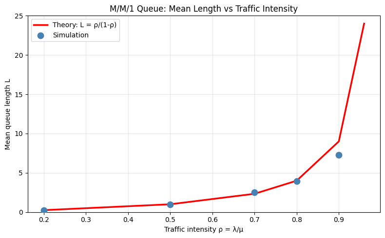
## 2. M/M/1 Queue
# Arrivals: Poisson(lambda). Service: Exp(mu). 1 server.
# Stability: rho = lambda/mu < 1.
# Exact results:
#   Mean queue length: L = rho / (1 - rho)
#   Mean waiting time: W = 1/(mu - lambda)  (Little's Law: L = lambda * W)

def simulate_mm1_queue(arrival_rate, service_rate, n_customers, rng):
    """Simulate M/M/1 queue and return waiting times.
    
    Args:
        arrival_rate: lambda (Poisson arrivals)
        service_rate: mu (Exponential service)
        n_customers: number of customers to simulate
        rng: numpy random generator
    
    Returns:
        waiting_times: time each customer waits in queue (before service)
        sojourn_times: total time in system (wait + service)
    """
    inter_arrivals = rng.exponential(1.0 / arrival_rate, n_customers)
    service_times = rng.exponential(1.0 / service_rate, n_customers)
    
    arrival_times = np.cumsum(inter_arrivals)
    waiting_times = np.zeros(n_customers)
    departure_times = np.zeros(n_customers)
    
    # Server is free at time 0
    server_free_at = 0.0
    
    for i in range(n_customers):
        service_start = max(arrival_times[i], server_free_at)
        waiting_times[i] = service_start - arrival_times[i]
        departure_times[i] = service_start + service_times[i]
        server_free_at = departure_times[i]
    
    sojourn_times = waiting_times + service_times
    return waiting_times, sojourn_times

mu = 5.0  # service rate
lambdas = [1.0, 2.5, 3.5, 4.0, 4.5, 4.8]
n_customers = 20_000

print(f"{'λ':>6} {'ρ':>6} {'L (sim)':>10} {'L (theory)':>12} {'W (sim)':>10} {'W (theory)':>12}")
print("-" * 62)

L_sim_list, L_theory_list, rho_list = [], [], []

for lam in lambdas:
    rho = lam / mu
    wait, sojourn = simulate_mm1_queue(lam, mu, n_customers, rng)
    
    # Little's Law: L = lambda * W
    W_sim = sojourn.mean()
    L_sim = lam * W_sim
    
    W_theory = 1 / (mu - lam)
    L_theory = rho / (1 - rho)
    
    L_sim_list.append(L_sim)
    L_theory_list.append(L_theory)
    rho_list.append(rho)
    
    print(f"{lam:>6.1f} {rho:>6.3f} {L_sim:>10.3f} {L_theory:>12.3f} {W_sim:>10.4f} {W_theory:>12.4f}")

fig, ax = plt.subplots(figsize=(8, 5))
ax.plot(rho_list, L_theory_list, 'r-', linewidth=2.5, label='Theory: L = ρ/(1-ρ)')
ax.scatter(rho_list, L_sim_list, color='steelblue', s=80, zorder=5,
           label='Simulation')
ax.set_xlabel('Traffic intensity ρ = λ/μ')
ax.set_ylabel('Mean queue length L')
ax.set_title('M/M/1 Queue: Mean Length vs Traffic Intensity')
ax.legend()
ax.grid(True, alpha=0.3)
ax.set_ylim(0, 25)
plt.tight_layout()
plt.savefig('mm1_queue.png', dpi=120, bbox_inches='tight')
plt.show()