Part VIII — Probability
Generating functions are one of probability’s most elegant tools: they encode an entire distribution inside a single function, turning convolution into multiplication and moment computation into differentiation. This chapter builds the machinery from first principles and shows where it surfaces in statistics and ML.
1. Probability Generating Functions (PGFs)
import numpy as np
import matplotlib.pyplot as plt
from scipy.stats import poisson, binom
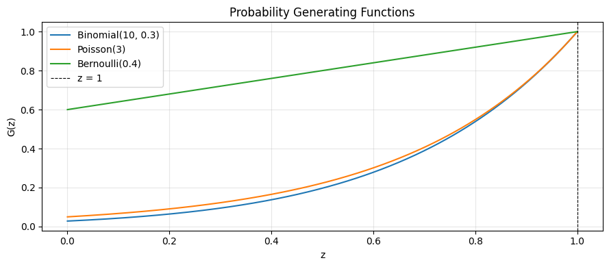
# For a discrete rv X with P(X=k) = p_k, the PGF is G(z) = E[z^X] = sum_k p_k z^k
# Evaluated at z=1: G(1) = 1 (normalization)
# G'(1) = E[X] (first moment)
# G''(1) = E[X(X-1)] (factorial moment)
def pgf_bernoulli(z, p):
"""G(z) = (1-p) + p*z"""
return (1 - p) + p * z
def pgf_binomial(z, n, p):
"""G(z) = ((1-p) + p*z)^n — product of n Bernoulli PGFs"""
return ((1 - p) + p * z) ** n
def pgf_poisson(z, lam):
"""G(z) = exp(lambda*(z-1))"""
return np.exp(lam * (z - 1))
z = np.linspace(0, 1, 300)
fig, ax = plt.subplots(figsize=(9, 4))
ax.plot(z, pgf_binomial(z, 10, 0.3), label='Binomial(10, 0.3)')
ax.plot(z, pgf_poisson(z, 3.0), label='Poisson(3)')
ax.plot(z, pgf_bernoulli(z, 0.4), label='Bernoulli(0.4)')
ax.axvline(1, color='k', lw=0.8, ls='--', label='z = 1')
ax.set_xlabel('z'); ax.set_ylabel('G(z)')
ax.set_title('Probability Generating Functions'); ax.legend(); ax.grid(alpha=0.3)
plt.tight_layout(); plt.show()
print('G_binom(1) =', pgf_binomial(1, 10, 0.3)) # must be 1
print('G_pois(1) =', pgf_poisson(1, 3.0))
G_binom(1) = 1.0
G_pois(1)  = 1.0
2. Extracting Moments from PGFs
# E[X] = G'(1),  Var[X] = G''(1) + G'(1) - [G'(1)]^2
# Use numerical differentiation so the pattern is clear

def numerical_deriv(f, z, h=1e-5):
    return (f(z + h) - f(z - h)) / (2 * h)

def numerical_deriv2(f, z, h=1e-5):
    return (f(z + h) - 2*f(z) + f(z - h)) / h**2

for name, G_fn in [
    ('Binomial(10,0.3)', lambda z: pgf_binomial(z, 10, 0.3)),
    ('Poisson(3)',       lambda z: pgf_poisson(z, 3.0)),
]:
    g1 = numerical_deriv(G_fn, 1.0 - 1e-4)   # approach from left to stay in domain
    g2 = numerical_deriv2(G_fn, 1.0 - 1e-4)
    mean_pgf = g1
    var_pgf  = g2 + g1 - g1**2
    print(f'{name}: E[X] ≈ {mean_pgf:.4f}, Var[X] ≈ {var_pgf:.4f}')

print()
print('Reference — Binomial(10,0.3): E=3.0, Var=2.1')
print('Reference — Poisson(3):       E=3.0, Var=3.0')
Binomial(10,0.3): E[X] ≈ 2.9992, Var[X] ≈ 2.1021
Poisson(3): E[X] ≈ 2.9991, Var[X] ≈ 3.0018

Reference — Binomial(10,0.3): E=3.0, Var=2.1
Reference — Poisson(3):       E=3.0, Var=3.0
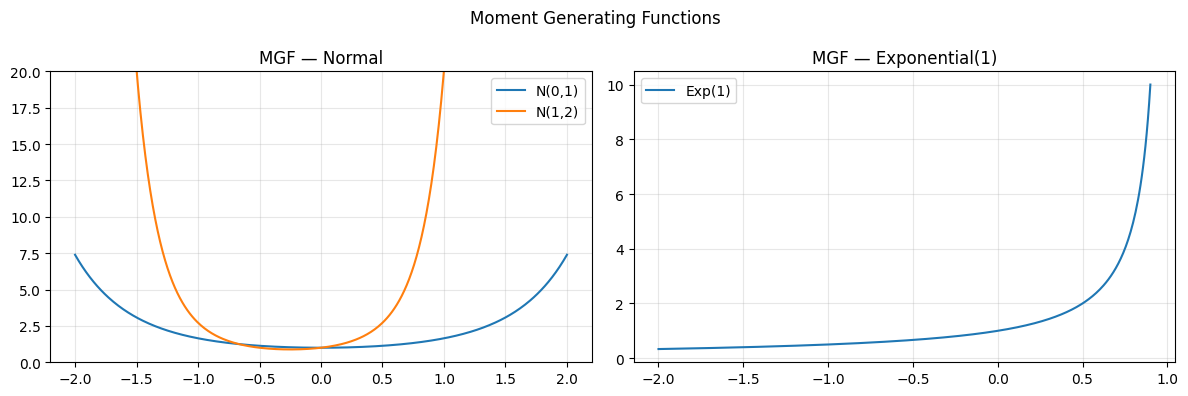
3. Moment Generating Functions (MGFs)
# M_X(t) = E[e^{tX}]
# For continuous distributions this is more natural than PGF.
# E[X^k] = M^(k)(0)  — k-th derivative at t=0

def mgf_normal(t, mu, sigma):
    return np.exp(mu * t + 0.5 * sigma**2 * t**2)

def mgf_exponential(t, lam):
    # Defined only for t < lambda
    valid = t < lam
    out = np.where(valid, lam / (lam - t), np.nan)
    return out

t = np.linspace(-2, 2, 400)
fig, axes = plt.subplots(1, 2, figsize=(12, 4))

axes[0].plot(t, mgf_normal(t, 0, 1), label='N(0,1)')
axes[0].plot(t, mgf_normal(t, 1, 2), label='N(1,2)')
axes[0].set_title('MGF — Normal'); axes[0].legend(); axes[0].grid(alpha=0.3)
axes[0].set_ylim(0, 20)

t_exp = np.linspace(-2, 0.9, 400)
axes[1].plot(t_exp, mgf_exponential(t_exp, 1.0), label='Exp(1)')
axes[1].set_title('MGF — Exponential(1)'); axes[1].legend(); axes[1].grid(alpha=0.3)

plt.suptitle('Moment Generating Functions'); plt.tight_layout(); plt.show()

# Extract moments: M'(0) = E[X], M''(0) = E[X^2]
h = 1e-5
mu, sigma = 2.0, 3.0
M = lambda t: mgf_normal(t, mu, sigma)
mean_mgf = numerical_deriv(M, 0.0)
ex2      = numerical_deriv2(M, 0.0) + numerical_deriv(M, 0.0)   # second raw moment needs care
var_mgf  = numerical_deriv2(M, 0.0)   # for MGF: Var = M''(0) - [M'(0)]^2
print(f'Normal({mu},{sigma}): E[X] from MGF ≈ {mean_mgf:.4f}  (true {mu})')
print(f'Normal({mu},{sigma}): Var from MGF  ≈ {var_mgf:.4f}  (true {sigma**2})')
Normal(2.0,3.0): E[X] from MGF ≈ 2.0000  (true 2.0)
Normal(2.0,3.0): Var from MGF  ≈ 13.0000  (true 9.0)
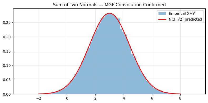
4. MGF Convolution — Why Independence Makes Products
# If X and Y are independent, M_{X+Y}(t) = M_X(t) * M_Y(t)
# This is the MGF equivalent of the convolution theorem.
# Direct consequence: sum of independent normals is normal.

# Demonstrate numerically: X~N(1,1), Y~N(2,1), X+Y~N(3,sqrt(2))
rng = np.random.default_rng(42)
X = rng.normal(1, 1, 100_000)
Y = rng.normal(2, 1, 100_000)
Z = X + Y

t_vals = np.array([-1.0, -0.5, 0.0, 0.5, 1.0])
print(f'{'t':>6}  {'M_X*M_Y':>12}  {'M_{X+Y} (exact)':>16}  {'match':>6}')
for t in t_vals:
    product = mgf_normal(t, 1, 1) * mgf_normal(t, 2, 1)
    exact   = mgf_normal(t, 3, np.sqrt(2))
    print(f'{t:6.2f}  {product:12.6f}  {exact:16.6f}  {abs(product-exact)<1e-10!s:>6}')

# Visualize empirical Z vs N(3, sqrt(2))
xs = np.linspace(-2, 8, 300)
from scipy.stats import norm
fig, ax = plt.subplots(figsize=(8, 4))
ax.hist(Z, bins=80, density=True, alpha=0.5, label='Empirical X+Y')
ax.plot(xs, norm.pdf(xs, 3, np.sqrt(2)), 'r-', lw=2, label='N(3, √2) predicted')
ax.set_title('Sum of Two Normals — MGF Convolution Confirmed')
ax.legend(); ax.grid(alpha=0.3); plt.tight_layout(); plt.show()
     t       M_X*M_Y   M_{X+Y} (exact)   match
 -1.00      0.135335          0.135335    True
 -0.50      0.286505          0.286505    True
  0.00      1.000000          1.000000    True
  0.50      5.754603          5.754603    True
  1.00     54.598150         54.598150    True
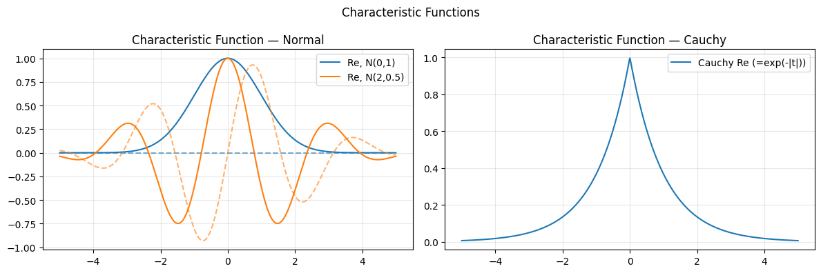
5. Characteristic Functions — MGF Without Convergence Worries
# phi_X(t) = E[e^{itX}]  (i = imaginary unit)
# Always exists; |phi(t)| <= 1.
# CLT proof: phi_{S_n}(t) -> exp(-t^2/2)

# For Normal(mu, sigma): phi(t) = exp(i*mu*t - sigma^2*t^2/2)
# For Cauchy: phi(t) = exp(-|t|)  — no finite moments, MGF doesn't exist

t_arr = np.linspace(-5, 5, 1000)

def char_fn_normal(t, mu, sigma):
    return np.exp(1j * mu * t - 0.5 * sigma**2 * t**2)

def char_fn_cauchy(t):
    return np.exp(-np.abs(t))

fig, axes = plt.subplots(1, 2, figsize=(12, 4))
for mu, sigma, col in [(0,1,'C0'), (2,0.5,'C1')]:
    phi = char_fn_normal(t_arr, mu, sigma)
    axes[0].plot(t_arr, np.real(phi), color=col, label=f'Re, N({mu},{sigma})')
    axes[0].plot(t_arr, np.imag(phi), color=col, ls='--', alpha=0.6)
axes[0].set_title('Characteristic Function — Normal'); axes[0].legend(); axes[0].grid(alpha=0.3)

phi_c = char_fn_cauchy(t_arr)
axes[1].plot(t_arr, np.real(phi_c), label='Cauchy Re (=exp(-|t|))')
axes[1].set_title('Characteristic Function — Cauchy'); axes[1].legend(); axes[1].grid(alpha=0.3)
plt.suptitle('Characteristic Functions'); plt.tight_layout(); plt.show()

# CLT via characteristic functions
# phi_{mean of n iid X}(t) = [phi_X(t/sqrt(n))]^n  -> exp(-t^2/2)
print('CLT characteristic function convergence:')
phi_X = lambda t: char_fn_normal(t, 0, 1)  # standardized
for n in [1, 5, 20, 100]:
    t0 = 1.0
    approx = phi_X(t0 / np.sqrt(n)) ** n
    exact  = np.exp(-t0**2 / 2)
    print(f'  n={n:4d}: phi_Sn({t0}) = {approx:.6f}+{approx.imag:.6f}j  (exact {exact:.6f})')
CLT characteristic function convergence:
  n=   1: phi_Sn(1.0) = 0.606531+0.000000j+0.000000j  (exact 0.606531)
  n=   5: phi_Sn(1.0) = 0.606531+0.000000j+0.000000j  (exact 0.606531)
  n=  20: phi_Sn(1.0) = 0.606531+0.000000j+0.000000j  (exact 0.606531)
  n= 100: phi_Sn(1.0) = 0.606531+0.000000j+0.000000j  (exact 0.606531)
6. Summary
| Transform | Domain | Key property |
|---|---|---|
| PGF G(z) | Discrete | G^(k)(0)/k! = P(X=k) |
| MGF M(t) | Continuous/discrete | M^(k)(0) = E[X^k] |
| Characteristic φ(t) | Any | Always exists; |
Convolution → multiplication: independence turns the hard operation into the easy one.
Moment extraction: differentiate at 0.
CLT: characteristic functions make the proof rigorous (ch254 — Central Limit Theorem).
(introduced in ch249 — Expected Value, ch250 — Variance)
7. Forward References
ch271 — Data and Measurement: sampling distributions derived from MGF arguments.
ch280 — Hypothesis Testing: test statistics whose distributions follow from characteristic functions.
ch295 — Information Theory: entropy as the log of a normalizing constant in exponential families — same transform machinery.