Part VIII - Probability
Independence is the exception, not the rule. Copulas separate marginal behavior from dependence, giving a modular way to build joint distributions. Sklar’s theorem guarantees this decomposition always exists.
1. Why Marginals Are Not Enough
import numpy as np
import matplotlib.pyplot as plt
from scipy.stats import norm, kendalltau, spearmanr

rng = np.random.default_rng(0)

n = 1000
Z1, Z2 = rng.multivariate_normal([0, 0], [[1, 0.9], [0.9, 1]], n).T
Z3, Z4 = rng.multivariate_normal([0, 0], [[1, -0.9], [-0.9, 1]], n).T
Z5 = rng.normal(0, 1, n); Z6 = rng.normal(0, 1, n)

fig, axes = plt.subplots(1, 3, figsize=(14, 4))
for ax, (X, Y), title in zip(axes,
        [(Z1, Z2), (Z3, Z4), (Z5, Z6)],
        ["Positive (rho~0.9)", "Negative (rho~-0.9)", "Independent"]):
    ax.scatter(X, Y, alpha=0.2, s=6, color="steelblue")
    ax.set_title(title); ax.set_xlabel("X"); ax.set_ylabel("Y"); ax.grid(alpha=0.3)
plt.suptitle("Same Marginals - Different Joint Structures", y=1.02)
plt.tight_layout(); plt.show()
print("All three datasets have marginals ~ N(0,1) but different joint structure.")
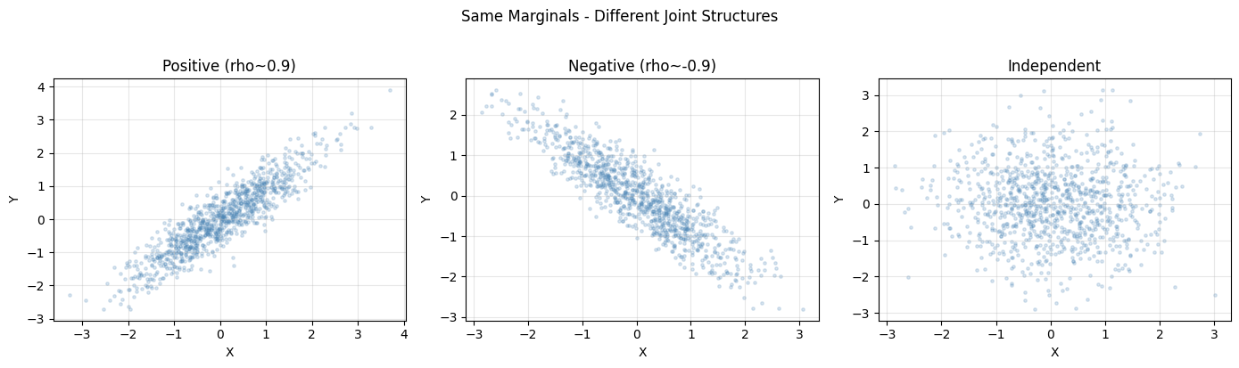
All three datasets have marginals ~ N(0,1) but different joint structure.
2. Sklar’s Theorem and the Copula
For any joint CDF H(x,y) with marginals F(x) and G(y), there exists a copula C such that H(x,y) = C(F(x), G(y)). Transform each marginal to Uniform[0,1] via the probability integral transform. What remains IS the copula.
def to_uniform(x):
    n = len(x)
    ranks = np.argsort(np.argsort(x))
    return (ranks + 1) / (n + 1)

U1 = to_uniform(Z1); U2 = to_uniform(Z2)
fig, axes = plt.subplots(1, 2, figsize=(11, 4))
axes[0].scatter(Z1, Z2, alpha=0.2, s=6)
axes[0].set_title("Original data - N(0,1) marginals")
axes[1].scatter(U1, U2, alpha=0.2, s=6)
axes[1].set_title("Copula space - U[0,1] marginals")
for ax in axes: ax.grid(alpha=0.3)
plt.tight_layout(); plt.show()
print("Copula space reveals pure dependence structure stripped of marginals.")
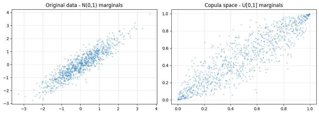
Copula space reveals pure dependence structure stripped of marginals.
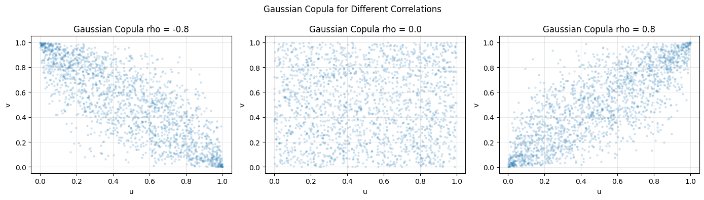
3. The Gaussian Copula
from scipy.stats import norm as snorm

def gaussian_copula_sample(n, rho, rng):
    Z = rng.multivariate_normal([0, 0], [[1, rho], [rho, 1]], n)
    U = snorm.cdf(Z[:, 0])
    V = snorm.cdf(Z[:, 1])
    return U, V

fig, axes = plt.subplots(1, 3, figsize=(14, 4))
for ax, rho in zip(axes, [-0.8, 0.0, 0.8]):
    U, V = gaussian_copula_sample(2000, rho, rng)
    ax.scatter(U, V, alpha=0.15, s=5)
    ax.set_title(f"Gaussian Copula rho = {rho}")
    ax.set_xlabel("u"); ax.set_ylabel("v"); ax.grid(alpha=0.3)
plt.suptitle("Gaussian Copula for Different Correlations")
plt.tight_layout(); plt.show()
4. The Clayton Copula - Tail Dependence
Clayton copula: C(u,v;theta) = (u^{-theta} + v^{-theta} - 1)^{-1/theta}. Exhibits lower-tail dependence. Used in credit risk modeling.
def clayton_copula_sample(n, theta, rng):
    u = rng.uniform(0, 1, n)
    p = rng.uniform(0, 1, n)
    # Closed-form inverse for Clayton conditional
    inner = p ** (-theta / (1 + theta)) - 1 + u ** theta
    inner = np.maximum(inner, 1e-12)
    v = inner ** (-1 / theta)
    return np.clip(u, 1e-9, 1-1e-9), np.clip(v, 1e-9, 1-1e-9)

fig, axes = plt.subplots(1, 3, figsize=(14, 4))
for ax, theta in zip(axes, [0.5, 2.0, 8.0]):
    U, V = clayton_copula_sample(3000, theta, rng)
    ax.scatter(U, V, alpha=0.1, s=4)
    ax.set_title(f"Clayton theta = {theta}")
    ax.set_xlabel("u"); ax.set_ylabel("v"); ax.grid(alpha=0.3)
plt.suptitle("Clayton Copula - Lower Tail Dependence")
plt.tight_layout(); plt.show()
print("Extreme values cluster in lower-left corner: lower tail dependence.")
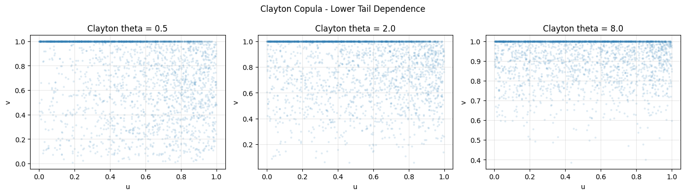
Extreme values cluster in lower-left corner: lower tail dependence.
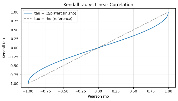
5. Rank Correlation: Kendall tau and Spearman rho
Pearson correlation measures linear dependence and changes with marginals. Rank correlations are copula properties - invariant to monotone marginal transformations.
rho_vals = np.linspace(-1, 1, 200)
tau_theory = 2 / np.pi * np.arcsin(rho_vals)
plt.figure(figsize=(7, 4))
plt.plot(rho_vals, tau_theory, label="tau = (2/pi)*arcsin(rho)")
plt.plot([-1, 1], [-1, 1], "k--", alpha=0.4, label="tau = rho (reference)")
plt.xlabel("Pearson rho"); plt.ylabel("Kendall tau")
plt.title("Kendall tau vs Linear Correlation"); plt.legend(); plt.grid(alpha=0.3)
plt.tight_layout(); plt.show()

for rho in [-0.8, 0.0, 0.5, 0.9]:
    U, V = gaussian_copula_sample(5000, rho, rng)
    tau_emp, _ = kendalltau(U, V)
    tau_pred   = 2 / np.pi * np.arcsin(rho)
    spr, _     = spearmanr(U, V)
    print(f"rho={rho:+.1f}  tau_predicted={tau_pred:+.4f}  tau_empirical={tau_emp:+.4f}  spearman={spr:+.4f}")
rho=-0.8  tau_predicted=-0.5903  tau_empirical=-0.5933  spearman=-0.7892
rho=+0.0  tau_predicted=+0.0000  tau_empirical=-0.0088  spearman=-0.0132
rho=+0.5  tau_predicted=+0.3333  tau_empirical=+0.3462  spearman=+0.4996
rho=+0.9  tau_predicted=+0.7129  tau_empirical=+0.7102  spearman=+0.8883
6. Building Joint Models with Custom Marginals
from scipy.stats import lognorm, expon

def joint_sample_via_copula(n, rho, rng):
    U, V = gaussian_copula_sample(n, rho, rng)
    X = lognorm.ppf(U, s=0.5, scale=1.0)
    Y = expon.ppf(V, scale=0.5)
    return X, Y

fig, axes = plt.subplots(1, 2, figsize=(12, 4))
for ax, rho, col in zip(axes, [-0.7, 0.7], ["steelblue", "darkorange"]):
    X, Y = joint_sample_via_copula(3000, rho, rng)
    ax.scatter(X, Y, alpha=0.15, s=5, color=col)
    ax.set_title(f"LogNormal x Exponential, rho = {rho}")
    ax.set_xlabel("LogNormal"); ax.set_ylabel("Exponential"); ax.grid(alpha=0.3)
plt.suptitle("Copula Construction with Custom Marginals")
plt.tight_layout(); plt.show()
print("Copula lets you combine ANY marginal distributions.")
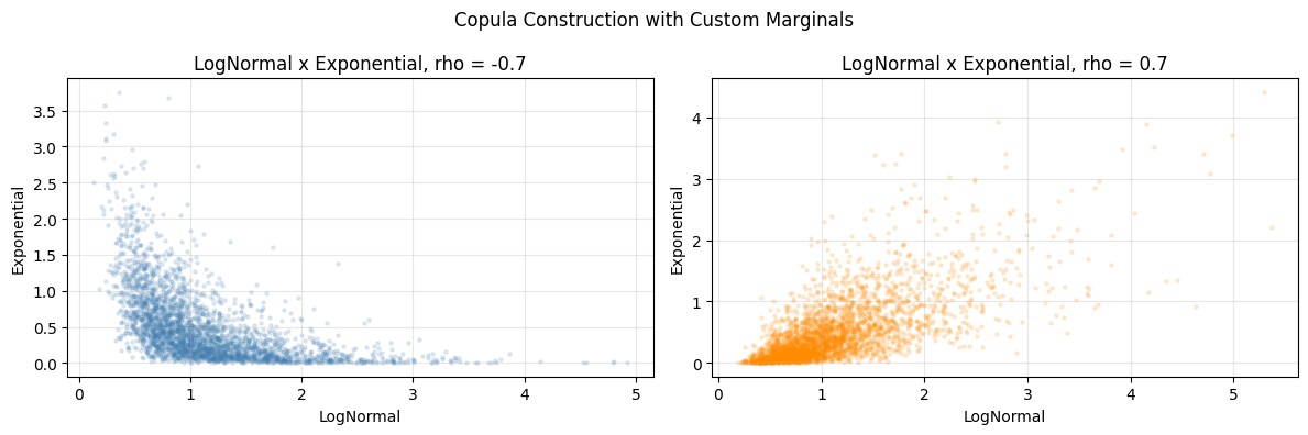
Copula lets you combine ANY marginal distributions.
7. Summary
Copulas decouple two questions:
What are the individual distributions? (marginals)
How do they co-move? (copula)
Rank correlations (Kendall tau, Spearman rho) are the natural summary statistics.
(builds on ch245 - Conditional Probability, ch247 - Random Variables)
8. Forward References
ch277 - Correlation: Pearson vs rank correlation in data analysis.
ch283 - Clustering: multivariate dependence in mixture models.
ch299 - Capstone: multivariate feature dependence in AI systems.