Part VIII - Probability
Single random variables are the building blocks. Machine learning deals with feature vectors, images, sequences: inherently multivariate objects. The multivariate normal is the workhorse, but its structure reveals principles that apply to any joint distribution.
1. Multivariate Normal - Setup and Sampling
import numpy as np
import matplotlib.pyplot as plt
from scipy.stats import multivariate_normal

rng = np.random.default_rng(42)

# Multivariate Normal: X ~ N(mu, Sigma)
# Key: covariance matrix Sigma must be positive semi-definite
mu = np.array([1.0, -0.5, 2.0])
Sigma = np.array([
    [2.0,  0.8, -0.3],
    [0.8,  1.5,  0.4],
    [-0.3, 0.4,  1.0]
])

samples = rng.multivariate_normal(mu, Sigma, 2000)
print(f"Shape: {samples.shape}")
print(f"Sample mean: {samples.mean(axis=0).round(3)}")
print(f"Sample cov:\n{np.cov(samples.T).round(3)}")
Shape: (2000, 3)
Sample mean: [ 0.959 -0.496  2.003]
Sample cov:
[[ 1.952  0.737 -0.262]
 [ 0.737  1.506  0.442]
 [-0.262  0.442  0.999]]
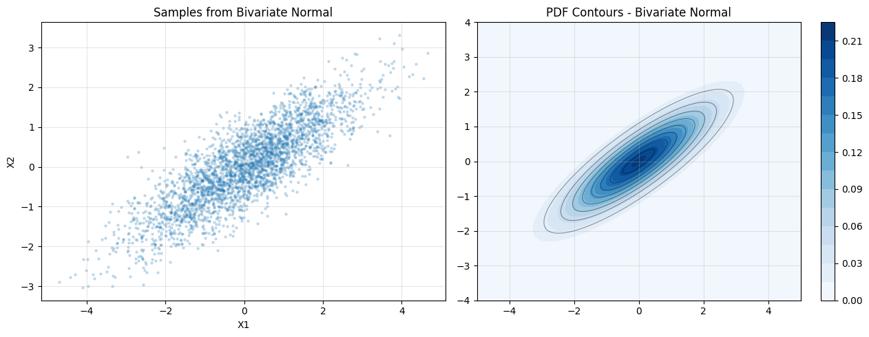
2. The Bivariate Case - Visualization
# 2D case for visualization
mu2 = np.array([0.0, 0.0])
Sigma2 = np.array([[2.0, 1.2], [1.2, 1.0]])
samples2 = rng.multivariate_normal(mu2, Sigma2, 3000)

x = np.linspace(-5, 5, 200)
y = np.linspace(-4, 4, 200)
X, Y = np.meshgrid(x, y)
pos = np.dstack([X, Y])
rv = multivariate_normal(mu2, Sigma2)
Z = rv.pdf(pos)

fig, axes = plt.subplots(1, 2, figsize=(13, 5))
axes[0].scatter(samples2[:, 0], samples2[:, 1], alpha=0.2, s=5)
axes[0].set_title("Samples from Bivariate Normal")
axes[0].set_xlabel("X1"); axes[0].set_ylabel("X2")

cnt = axes[1].contourf(X, Y, Z, levels=20, cmap="Blues")
axes[1].contour(X, Y, Z, levels=8, colors="k", alpha=0.4, linewidths=0.8)
plt.colorbar(cnt, ax=axes[1])
axes[1].set_title("PDF Contours - Bivariate Normal")
for ax in axes: ax.grid(alpha=0.3)
plt.tight_layout(); plt.show()
3. Conditional Distributions
A key property of the multivariate normal: all conditional and marginal distributions are themselves normal. The conditioning operation shifts the mean and reduces variance.
# Marginals and conditionals of multivariate normal are themselves normal.
# If X = [X1, X2] with mean [mu1, mu2] and cov [[S11, S12], [S21, S22]]:
# Conditional: X1 | X2=x2 ~ N(mu1 + S12/S22*(x2-mu2), S11 - S12^2/S22)

mu1, mu2_s = 0.0, 0.0
S11, S12, S22 = 2.0, 1.2, 1.0
x2_vals = [-2.0, 0.0, 2.0]

x1_grid = np.linspace(-5, 5, 300)
fig, ax = plt.subplots(figsize=(9, 5))

from scipy.stats import norm
for x2v in x2_vals:
    cond_mean = mu1 + S12 / S22 * (x2v - mu2_s)
    cond_var  = S11 - S12**2 / S22
    cond_std  = np.sqrt(cond_var)
    ax.plot(x1_grid, norm.pdf(x1_grid, cond_mean, cond_std),
            label=f"X1 | X2={x2v:.1f}: mean={cond_mean:.2f}, var={cond_var:.2f}")

ax.set_xlabel("X1"); ax.set_ylabel("PDF")
ax.set_title("Conditional Distributions: X1 | X2 = x2")
ax.legend(); ax.grid(alpha=0.3)
plt.tight_layout(); plt.show()
print(f"Marginal variance of X1: {S11} (unchanged regardless of conditioning value)")
print(f"Conditional variance: {S11 - S12**2/S22:.4f} (always smaller than marginal)")
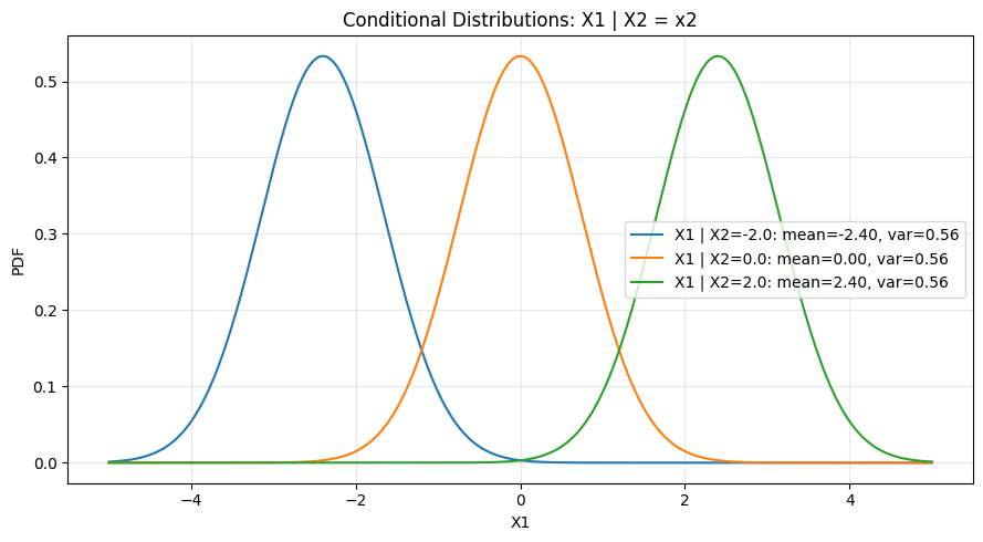
Marginal variance of X1: 2.0 (unchanged regardless of conditioning value)
Conditional variance: 0.5600 (always smaller than marginal)
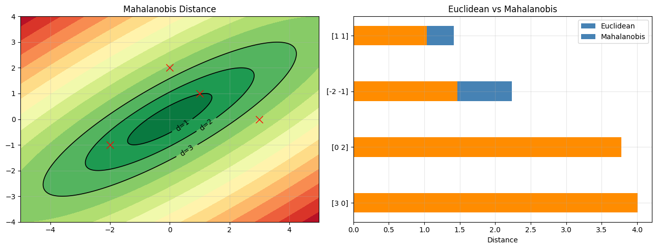
4. Mahalanobis Distance
The Mahalanobis distance accounts for correlation and scale. It is the natural distance metric in the space defined by the covariance structure. (Sigma^{-1} introduced in ch157 - Matrix Inverse)
# Mahalanobis distance: generalization of z-score to multiple dimensions
# d^2(x, mu) = (x - mu)^T Sigma^{-1} (x - mu)
# Contours of constant Mahalanobis distance are ellipses aligned to Sigma.

Sigma_inv = np.linalg.inv(Sigma2)

def mahalanobis(x, mu, Sigma_inv):
    diff = x - mu
    return np.sqrt(diff @ Sigma_inv @ diff)

# Compute for grid
dists = np.array([[mahalanobis(np.array([xi, yi]), mu2, Sigma_inv)
                   for xi in x] for yi in y])

fig, axes = plt.subplots(1, 2, figsize=(13, 5))
axes[0].contourf(X, Y, dists, levels=15, cmap="RdYlGn_r")
axes[0].set_title("Mahalanobis Distance")
c0 = axes[0].contour(X, Y, dists, levels=[1, 2, 3], colors="k", linewidths=1.2)
axes[0].clabel(c0, fmt="d=%.0f")

# Compare: Euclidean vs Mahalanobis for point classification
test_points = np.array([[3, 0], [0, 2], [-2, -1], [1, 1]])
for pt in test_points:
    mah = mahalanobis(pt.astype(float), mu2, Sigma_inv)
    euc = np.linalg.norm(pt - mu2)
    axes[0].plot(*pt, "rx", ms=10)
    axes[1].barh(str(pt), [euc, mah], 0.35,
                 color=["steelblue", "darkorange"])
axes[1].set_xlabel("Distance"); axes[1].set_title("Euclidean vs Mahalanobis")
axes[1].legend(["Euclidean", "Mahalanobis"])
for ax in axes: ax.grid(alpha=0.3)
plt.tight_layout(); plt.show()
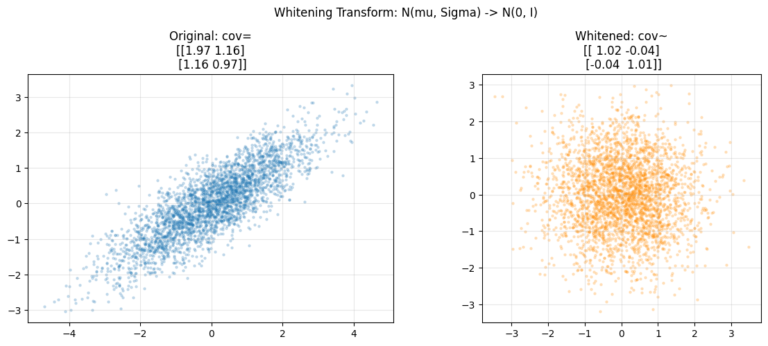
5. Whitening Transform
Whitening maps any multivariate normal to N(0, I). This is foundational preprocessing: removes correlations and equalizes scales. (Eigendecomposition from ch167 - Eigenvectors)
# Whitening transform: decorrelate and standardize
# W = Sigma^{-1/2} maps N(mu, Sigma) to N(0, I)

eigenvalues, eigenvectors = np.linalg.eigh(Sigma2)
Sigma_sqrt_inv = eigenvectors @ np.diag(1.0 / np.sqrt(eigenvalues)) @ eigenvectors.T

whitened = (samples2 - mu2) @ Sigma_sqrt_inv.T

fig, axes = plt.subplots(1, 2, figsize=(12, 5))
axes[0].scatter(samples2[:, 0], samples2[:, 1], alpha=0.2, s=5)
axes[0].set_title(f"Original: cov=\n{np.cov(samples2.T).round(2)}")
axes[0].set_aspect("equal")
axes[1].scatter(whitened[:, 0], whitened[:, 1], alpha=0.2, s=5, color="darkorange")
axes[1].set_title(f"Whitened: cov~\n{np.cov(whitened.T).round(2)}")
axes[1].set_aspect("equal")
for ax in axes: ax.grid(alpha=0.3)
plt.suptitle("Whitening Transform: N(mu, Sigma) -> N(0, I)")
plt.tight_layout(); plt.show()

print("Whitening is used in PCA preprocessing (introduced in ch175 - PCA)")
print("and in natural gradient methods in ML optimization.")
Whitening is used in PCA preprocessing (introduced in ch175 - PCA)
and in natural gradient methods in ML optimization.
6. Gaussian Processes - Infinite-Dimensional Extension
# Simulation: Gaussian process prior (1D, finite approximation)
# GP is an infinite-dimensional multivariate normal over functions.

def rbf_kernel(x1, x2, length_scale=1.0, amplitude=1.0):
    dist_sq = (x1[:, None] - x2[None, :]) ** 2
    return amplitude**2 * np.exp(-0.5 * dist_sq / length_scale**2)

x_grid = np.linspace(0, 5, 100)
n_samples_gp = 5

fig, axes = plt.subplots(1, 2, figsize=(13, 5))
for ax, ls, title in zip(axes, [0.3, 2.0], ["Short length scale (wiggly)", "Long length scale (smooth)"]):
    K = rbf_kernel(x_grid, x_grid, length_scale=ls)
    K += 1e-6 * np.eye(len(x_grid))   # jitter for numerical stability
    gp_samples = rng.multivariate_normal(np.zeros(len(x_grid)), K, n_samples_gp)
    for s in gp_samples:
        ax.plot(x_grid, s, alpha=0.7)
    ax.set_title(f"GP Prior Samples - {title}")
    ax.set_xlabel("x"); ax.set_ylabel("f(x)"); ax.grid(alpha=0.3)
plt.suptitle("Gaussian Process: Multivariate Normal over Functions")
plt.tight_layout(); plt.show()
print("GPs provide a Bayesian non-parametric approach to function estimation.")
print("Used in Bayesian optimization and spatial statistics (Kriging).")
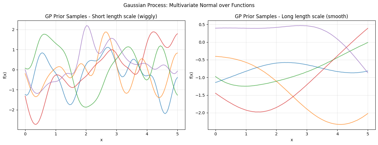
GPs provide a Bayesian non-parametric approach to function estimation.
Used in Bayesian optimization and spatial statistics (Kriging).
7. Summary
The multivariate normal is parameterized by mean vector mu and covariance matrix Sigma. Key operations:
Marginals: project out dimensions
Conditionals: slice with reduced variance
Mahalanobis: distance respecting covariance
Whitening: decorrelate to isotropic space
(builds on ch247 - Random Variables, ch250 - Variance, ch175 - PCA)
8. Forward References
ch277 - Correlation: correlation as normalized covariance in data pipelines.
ch287 - Clustering: Gaussian mixture models use multivariate normals per cluster.
ch295 - Neural Network Math Review: weight initialization and batch normalization.