ch286 — Bayesian Statistics - Mathematics for Programmers

(Applies Bayes’ theorem from ch246; connects to prior knowledge and posterior updates)

1. The Bayesian View¶

Frequentist statistics treats parameters as fixed unknowns. Bayesian statistics treats parameters as random variables with probability distributions that encode uncertainty.

Before seeing data, you have a prior belief about a parameter $\theta$ . After seeing data $D$ , you update to a posterior:

\underbrace{P(\theta \mid D)}_{\text{posterior}} = \frac{\underbrace{P(D \mid \theta)}_{\text{likelihood}} \cdot \underbrace{P(\theta)}_{\text{prior}}}{\underbrace{P(D)}_{\text{normalizer}}}

(1)

(Bayes’ theorem was introduced in ch246.)

The posterior is the complete answer: it is a distribution over all plausible parameter values given your data and prior beliefs.

2. Beta-Binomial: Bayesian A/B Testing¶

import numpy as np
import matplotlib.pyplot as plt
from scipy import stats

rng = np.random.default_rng(42)

# Beta distribution: conjugate prior for binomial likelihood
# Prior: Beta(alpha, beta) encodes prior belief about conversion rate p
# Posterior: Beta(alpha + successes, beta + failures) -- exact, closed form

def bayesian_ab_test(
    n_control:   int, k_control:   int,   # trials, successes
    n_treatment: int, k_treatment: int,
    prior_alpha: float = 1.0,             # Beta(1,1) = uniform prior
    prior_beta:  float = 1.0,
    n_samples:   int   = 100_000,
    rng = None,
) -> dict:
    """
    Bayesian comparison of two conversion rates.
    Uses Beta-Binomial conjugate model.
    Returns posterior samples and probability that treatment > control.
    """
    if rng is None: rng = np.random.default_rng()

    # Posterior parameters
    a_c = prior_alpha + k_control
    b_c = prior_beta  + (n_control - k_control)
    a_t = prior_alpha + k_treatment
    b_t = prior_beta  + (n_treatment - k_treatment)

    # Sample from posteriors
    samples_c = rng.beta(a_c, b_c, n_samples)
    samples_t = rng.beta(a_t, b_t, n_samples)

    prob_treatment_wins = np.mean(samples_t > samples_c)
    expected_lift       = np.mean(samples_t - samples_c)

    # 95% credible interval for the difference
    diff_samples = samples_t - samples_c
    ci_lo, ci_hi = np.percentile(diff_samples, [2.5, 97.5])

    return {
        'posterior_control':   (a_c, b_c),
        'posterior_treatment': (a_t, b_t),
        'samples_c':   samples_c,
        'samples_t':   samples_t,
        'prob_t_wins': prob_treatment_wins,
        'expected_lift': expected_lift,
        'credible_interval_95': (ci_lo, ci_hi),
    }


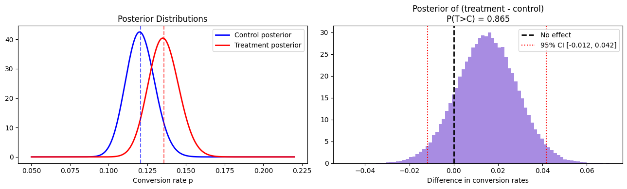
# Example: 1200 control, 144 conversions (12%)
#          1200 treatment, 162 conversions (13.5%)
result = bayesian_ab_test(
    n_control=1200,   k_control=144,
    n_treatment=1200, k_treatment=162,
    rng=rng
)

print(f"P(treatment > control): {result['prob_t_wins']:.4f}")
print(f"Expected lift:          {result['expected_lift']:+.4f}")
print(f"95% credible interval:  [{result['credible_interval_95'][0]:+.4f}, "
      f"{result['credible_interval_95'][1]:+.4f}]")

# Visualize posteriors
x = np.linspace(0.05, 0.22, 500)
a_c, b_c = result['posterior_control']
a_t, b_t = result['posterior_treatment']

fig, axes = plt.subplots(1, 2, figsize=(13, 4))

ax = axes[0]
ax.plot(x, stats.beta.pdf(x, a_c, b_c), 'b-', lw=2, label='Control posterior')
ax.plot(x, stats.beta.pdf(x, a_t, b_t), 'r-', lw=2, label='Treatment posterior')
ax.axvline(a_c/(a_c+b_c), color='blue', ls='--', alpha=0.6)
ax.axvline(a_t/(a_t+b_t), color='red',  ls='--', alpha=0.6)
ax.set_xlabel('Conversion rate p')
ax.set_title('Posterior Distributions')
ax.legend()

ax = axes[1]
diff = result['samples_t'] - result['samples_c']
ax.hist(diff, bins=80, color='mediumpurple', edgecolor='none', density=True, alpha=0.8)
ax.axvline(0, color='black', lw=2, ls='--', label='No effect')
lo, hi = result['credible_interval_95']
ax.axvline(lo, color='red', lw=1.5, ls=':', label=f'95% CI [{lo:.3f}, {hi:.3f}]')
ax.axvline(hi, color='red', lw=1.5, ls=':')
pwin = result['prob_t_wins']
ax.fill_between(
    np.linspace(lo, hi, 100),
    np.zeros(100), np.interp(np.linspace(lo, hi, 100),
                              np.sort(diff),
                              np.linspace(0, 1, len(diff))), alpha=0
)
ax.set_title(f'Posterior of (treatment - control)\nP(T>C) = {pwin:.3f}')
ax.set_xlabel('Difference in conversion rates')
ax.legend()

plt.tight_layout()
plt.show()

P(treatment > control): 0.8651
Expected lift:          +0.0150
95% credible interval:  [-0.0118, +0.0418]

3. Prior Sensitivity¶

# How much does the prior affect the posterior?
# Large data: prior barely matters. Small data: prior dominates.

priors = [
    (1, 1,   'Uniform prior Beta(1,1)'),
    (10, 80, 'Informative: strong belief p≈0.11'),
    (50, 50, 'Strong: believes p=0.5'),
]

# Small experiment: 30 obs, 5 successes
n_obs, k_obs = 30, 5

x = np.linspace(0, 0.5, 500)
fig, axes = plt.subplots(1, 2, figsize=(13, 4))

for ax, n_data, k_data, title in [
    (axes[0], 30, 5, f'Small data (n={30}, k={5})'),
    (axes[1], 3000, 500, f'Large data (n={3000}, k={500})'),
]:
    for a_p, b_p, label in priors:
        a_post = a_p + k_data
        b_post = b_p + (n_data - k_data)
        ax.plot(x, stats.beta.pdf(x, a_post, b_post), lw=2, label=label)

    ax.axvline(k_data/n_data, color='black', ls='--', lw=2, label='MLE (data only)')
    ax.set_title(title); ax.set_xlabel('p'); ax.legend(fontsize=7)

plt.suptitle('Prior Sensitivity — Small vs Large Data', fontsize=11)
plt.tight_layout()
plt.show()

print("With 30 obs: posteriors differ substantially across priors.")
print("With 3000 obs: posteriors converge regardless of prior.")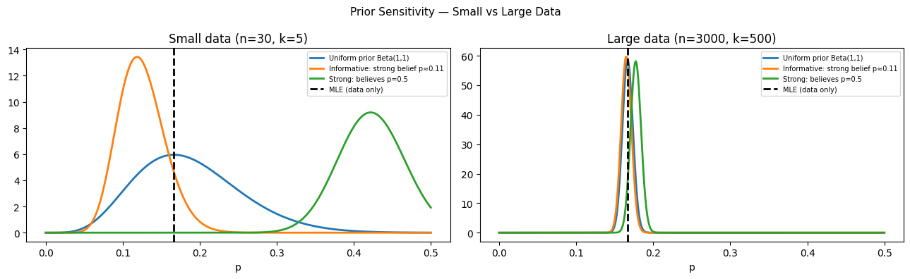

With 30 obs: posteriors differ substantially across priors.
With 3000 obs: posteriors converge regardless of prior.

4. Bayesian Updating Sequentially¶

# Sequential Bayesian update: no peeking problem
# Posterior after n observations = prior for observation n+1

true_p = 0.15
n_total = 500
observations = rng.binomial(1, true_p, n_total)

# Track posterior mean and 95% CI over time
a, b_par = 1.0, 1.0  # uniform prior
check_ns = [10, 30, 100, 200, 500]

fig, axes = plt.subplots(1, 5, figsize=(18, 3))
x = np.linspace(0, 0.4, 300)

k = 0
for i, ax in enumerate(axes):
    n_shown = check_ns[i]
    k = observations[:n_shown].sum()
    a_post = a + k
    b_post = b_par + (n_shown - k)
    post_mean = a_post / (a_post + b_post)
    ci = stats.beta.ppf([0.025, 0.975], a_post, b_post)

    ax.plot(x, stats.beta.pdf(x, a_post, b_post), 'b-', lw=2)
    ax.axvline(true_p, color='red', ls='--', lw=2, label='True p')
    ax.fill_between(x[(x>=ci[0]) & (x<=ci[1])],
                    stats.beta.pdf(x[(x>=ci[0]) & (x<=ci[1])], a_post, b_post),
                    alpha=0.3, color='blue')
    ax.set_title(f'n={n_shown}\nmean={post_mean:.3f}\n95%CI=[{ci[0]:.3f},{ci[1]:.3f}]', fontsize=8)
    ax.set_xlabel('p')
    if i == 0: ax.legend(fontsize=7)

plt.suptitle('Sequential Bayesian Update — Posterior Narrows with Data', fontsize=11)
plt.tight_layout()
plt.show()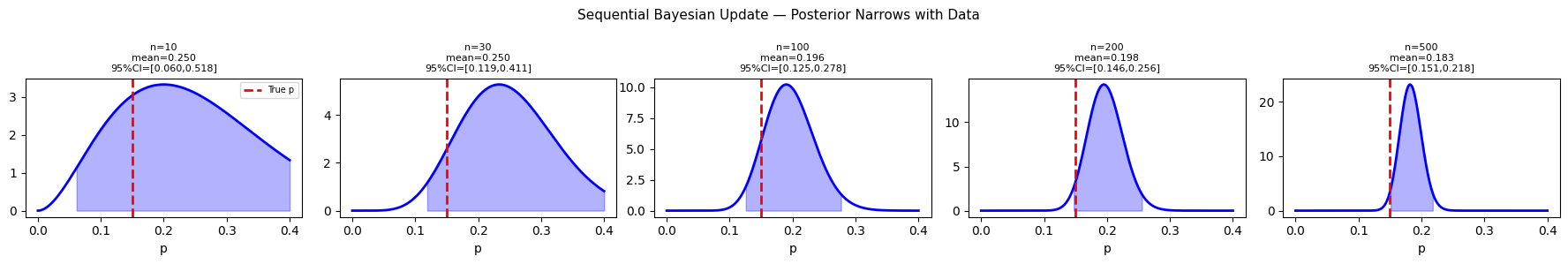

5. What Comes Next¶

Bayesian statistics provides the framework. ch287 — Information Theory provides a complementary lens: instead of asking how uncertain we are about a parameter, it asks how much information a random variable carries. The two frameworks connect deeply: entropy (ch288) is the log of the number of bits needed to encode a distribution, and KL divergence (ch289) measures how much information is lost when using one distribution to approximate another — the same loss minimized during training of most ML models.