Prerequisites: ch055 (Inverse Functions), ch063 (Step Functions)
You will learn:
Define sigmoid functions and their key properties
Derive logistic function from logit transform
Understand why sigmoid smoothly approximates the step function
Connect sigmoid to probability, log-odds, and logistic regression
Environment: Python 3.x, numpy, matplotlib
1. Concept
A sigmoid function is any function shaped like the letter S: monotonically increasing, bounded above and below, with an inflection point in the middle.
The most common is the logistic function: σ(x) = 1 / (1 + e^(-x))
Properties:
σ(x) ∈ (0, 1) for all x ∈ ℝ
σ(0) = 0.5
σ(-x) = 1 - σ(x) (antisymmetric around (0, 0.5))
σ’(x) = σ(x)(1 - σ(x)) — the derivative is expressible in terms of itself
lim_{x→+∞} σ(x) = 1, lim_{x→-∞} σ(x) = 0
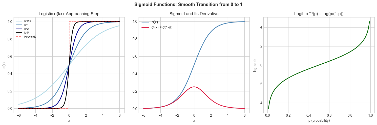
The sigmoid smooths the Heaviside step function. As a parameter k increases in 1/(1+e^(-kx)), the curve steepens toward a step at x=0.
Logit (inverse sigmoid): logit(p) = log(p/(1-p)) — converts probability to log-odds. σ and logit are inverses (introduced in ch055).
2. Intuition & Mental Models
Physical analogy: A dimmer switch. A step switch is on or off. A sigmoid dimmer smoothly transitions from fully off (0) to fully on (1). The steepness parameter k controls how sharp the transition is.
Computational analogy: In logistic regression, σ(wᵀx + b) outputs a probability. The sigmoid converts an unbounded linear score into a bounded [0,1] probability. That’s its exact role in the model.
Recall from ch063 (Step Functions): Heaviside is the limiting case of sigmoid as steepness → ∞.
3. Visualization
# --- Visualization: Sigmoid family and steepness ---
import numpy as np
import matplotlib.pyplot as plt
plt.style.use('seaborn-v0_8-whitegrid')

x = np.linspace(-6, 6, 500)

def logistic(x, k=1): return 1 / (1 + np.exp(-k * x))
def tanh_norm(x): return (np.tanh(x) + 1) / 2  # shifted to [0,1]

fig, axes = plt.subplots(1, 3, figsize=(15, 5))

# Effect of steepness
for k, color in zip([0.5, 1, 2, 5], ['lightblue','steelblue','darkblue','black']):
    axes[0].plot(x, logistic(x, k), color=color, linewidth=2, label=f'k={k}')
axes[0].plot(x, np.where(x>=0, 1, 0), 'r--', linewidth=1.5, alpha=0.5, label='Heaviside')
axes[0].set_title('Logistic σ(kx): Approaching Step')
axes[0].set_xlabel('x'); axes[0].set_ylabel('σ(x)')
axes[0].legend(fontsize=8)

# Derivative
sx = logistic(x)
axes[1].plot(x, sx, color='steelblue', linewidth=2, label='σ(x)')
axes[1].plot(x, sx*(1-sx), color='crimson', linewidth=2, label="σ'(x) = σ(1-σ)")
axes[1].set_title("Sigmoid and Its Derivative")
axes[1].set_xlabel('x'); axes[1].legend()

# Logit (inverse)
p = np.linspace(0.01, 0.99, 500)
axes[2].plot(p, np.log(p/(1-p)), color='darkgreen', linewidth=2)
axes[2].axhline(0, color='black', linewidth=0.5)
axes[2].set_title('Logit: σ⁻¹(p) = log(p/(1-p))')
axes[2].set_xlabel('p (probability)'); axes[2].set_ylabel('log-odds')

plt.suptitle('Sigmoid Functions: Smooth Transition from 0 to 1', fontsize=13, fontweight='bold')
plt.tight_layout()
plt.show()
C:\Users\user\AppData\Local\Temp\ipykernel_11788\1138602643.py:36: UserWarning: Glyph 8315 (\N{SUPERSCRIPT MINUS}) missing from font(s) Arial.
plt.tight_layout()
c:\Users\user\OneDrive\Documents\book\.venv\Lib\site-packages\IPython\core\pylabtools.py:170: UserWarning: Glyph 8315 (\N{SUPERSCRIPT MINUS}) missing from font(s) Arial.
fig.canvas.print_figure(bytes_io, **kw)
4. Mathematical Formulation
Logistic sigmoid: σ(x) = 1/(1 + e^(-x))
Key identity: σ’(x) = σ(x)·(1 - σ(x)) This makes gradient computation in logistic regression and neural networks particularly clean.
Logit (inverse): logit(p) = ln(p/(1-p)) = ln(p) - ln(1-p)
Probability interpretation: If x = log-odds = ln(P/(1-P)), then σ(x) = P.
tanh relationship: tanh(x) = 2σ(2x) - 1 — tanh is a rescaled sigmoid
# --- Implementation: Numerically stable sigmoid ---
import numpy as np

def sigmoid(x):
    """
    Numerically stable sigmoid: 1 / (1 + e^(-x)).
    Avoids overflow for large negative x.

    Args:
        x: np.ndarray or scalar
    Returns:
        sigmoid values in (0, 1)
    """
    x = np.asarray(x, dtype=float)
    # For large positive x, use 1 - sigmoid(-x) to avoid exp overflow
    return np.where(x >= 0,
                    1 / (1 + np.exp(-x)),
                    np.exp(x) / (1 + np.exp(x)))

def sigmoid_derivative(x):
    """σ'(x) = σ(x)(1 - σ(x))."""
    s = sigmoid(x)
    return s * (1 - s)

def logit(p, eps=1e-7):
    """Inverse sigmoid: ln(p/(1-p)). Clips to avoid log(0)."""
    p = np.clip(p, eps, 1 - eps)
    return np.log(p / (1 - p))

# Verify round-trip
x_test = np.array([-5, -2, 0, 2, 5])
p_test = sigmoid(x_test)
x_recovered = logit(p_test)
print("x:          ", x_test)
print("σ(x):       ", p_test.round(4))
print("logit(σ(x)):", x_recovered.round(4))
print("Stable for large |x|:", sigmoid(np.array([-1000., 1000.]))  )
x: [-5 -2 0 2 5]
σ(x): [0.0067 0.1192 0.5 0.8808 0.9933]
logit(σ(x)): [-5. -2. 0. 2. 5.]
Stable for large |x|: [0. 1.]
C:\Users\user\AppData\Local\Temp\ipykernel_11788\2494554253.py:17: RuntimeWarning: overflow encountered in exp
  1 / (1 + np.exp(-x)),
C:\Users\user\AppData\Local\Temp\ipykernel_11788\2494554253.py:18: RuntimeWarning: overflow encountered in exp
  np.exp(x) / (1 + np.exp(x)))
C:\Users\user\AppData\Local\Temp\ipykernel_11788\2494554253.py:18: RuntimeWarning: invalid value encountered in divide
  np.exp(x) / (1 + np.exp(x)))
6. Experiments
Experiment 1: Plot σ(x) and σ’(x) together. Note that σ’(x) is maximized at x=0 where σ=0.5. This means gradients are largest at σ=0.5 and vanish near 0 or 1 — this is the ‘vanishing gradient’ problem in deep networks.
Experiment 2: Compare sigmoid to a piecewise linear approximation: max(0, min(1, x/4 + 0.5)). They look similar but behave differently at extremes.
7. Exercises
Easy 1. Compute σ(0), σ(1), σ(-1), σ(10), σ(-10) by hand and verify with code. (Expected: 0.5, 0.731, 0.269, ≈1, ≈0)
Easy 2. Verify the identity tanh(x) = 2σ(2x) - 1 numerically for x ∈ {-2, -1, 0, 1, 2}.
Medium 1. Implement logistic regression prediction: given weight vector w, bias b, and input matrix X (n×d), compute σ(X @ w + b). Apply to a 2-class dataset and visualize the decision boundary.
Medium 2. The softmax function generalizes sigmoid to K classes: softmax(x)ᵢ = e^xᵢ / Σⱼ e^xʲ. Implement a numerically stable version (subtract max before exponentiating). Verify outputs sum to 1.
Hard. Derive the gradient of binary cross-entropy loss L = -[y·log σ(x) + (1-y)·log(1-σ(x))] with respect to x. Show that ∂L/∂x = σ(x) - y. Verify numerically with finite differences.
9. Chapter Summary & Connections
Logistic sigmoid σ(x) = 1/(1+e^(-x)): smooth, bounded in (0,1)
σ’(x) = σ(x)(1-σ(x)): elegant self-referential derivative
Logit is the inverse: converts probability to log-odds
Sigmoid smoothly approximates the step function as steepness increases
Forward connections:
ch065 (Activation Functions) catalogs the full ML activation function family
Logistic regression in ch229 uses sigmoid as its core prediction function
Vanishing gradients in deep networks (ch216) are caused by sigmoid saturation