Prerequisites: ch062–064 (Piecewise, Step, Sigmoid)
You will learn:
Catalog the major activation functions used in neural networks
Understand why nonlinear activations are necessary
Compare saturating vs non-saturating activations
Implement and benchmark common activations
Environment: Python 3.x, numpy, matplotlib
1. Concept
Without activation functions, a multi-layer neural network collapses to a single linear transformation. Activation functions introduce nonlinearity — the capacity to model complex, non-linear relationships.
The major families:
Sigmoid / Tanh: saturating, bounded. Risk: vanishing gradients for large |x|
ReLU (Rectified Linear Unit): max(0, x). Non-saturating for x>0. Simple and effective
Leaky ReLU, ELU, SELU: fix the ‘dying ReLU’ problem (neurons stuck at 0)
GELU, Swish: smooth approximations to ReLU; used in transformers
Softmax: multi-class probability output layer
Dying ReLU problem: if a neuron receives only negative inputs, it outputs 0 and has zero gradient — it never updates. Leaky ReLU (α·x for x<0) fixes this by keeping a small gradient for negative inputs.
(Sigmoid introduced in ch064; piecewise structure from ch062)
2. Intuition & Mental Models
Physical analogy: Transistors in electronics. A transistor with no threshold is a linear amplifier. Add a threshold (saturation) and you get nonlinear logic gates. Neural networks are the mathematical equivalent — stacked nonlinear gates.
Computational analogy: Activation functions are the “decision units” of a network. Without them, no matter how many layers you stack, the output is just a matrix product of the input — expressible as a single linear transform.
3. Visualization
# --- Visualization: Activation function comparison ---
import numpy as np
import matplotlib.pyplot as plt
plt.style.use('seaborn-v0_8-whitegrid')

x = np.linspace(-4, 4, 500)

def relu(x): return np.maximum(0, x)
def leaky_relu(x, a=0.1): return np.where(x >= 0, x, a * x)
def elu(x, a=1.0): return np.where(x >= 0, x, a * (np.exp(x) - 1))
def sigmoid(x): return 1 / (1 + np.exp(-x))
def tanh(x): return np.tanh(x)
def gelu(x): return x * sigmoid(1.702 * x)  # fast approx
def swish(x): return x * sigmoid(x)

activations = [
    ('ReLU', relu, 'steelblue'),
    ('Leaky ReLU', leaky_relu, 'crimson'),
    ('ELU', elu, 'darkgreen'),
    ('Sigmoid', sigmoid, 'darkorange'),
    ('Tanh', tanh, 'purple'),
    ('GELU', gelu, 'brown'),
]

fig, axes = plt.subplots(2, 3, figsize=(15, 8))
for ax, (name, fn, color) in zip(axes.flat, activations):
    y = fn(x)
    dy = np.gradient(y, x)  # numerical derivative
    ax.plot(x, y, color=color, linewidth=2.5, label=name)
    ax.plot(x, dy, color=color, linewidth=1.5, linestyle='--', alpha=0.6, label=f"{name}'")
    ax.axhline(0, color='black', linewidth=0.4)
    ax.axvline(0, color='black', linewidth=0.4)
    ax.set_title(name)
    ax.set_xlabel('x'); ax.set_ylabel('f(x)')
    ax.set_ylim(-2, 4)
    ax.legend(fontsize=8)

plt.suptitle('Neural Network Activation Functions (solid=value, dashed=gradient)', fontsize=13, fontweight='bold')
plt.tight_layout()
plt.show()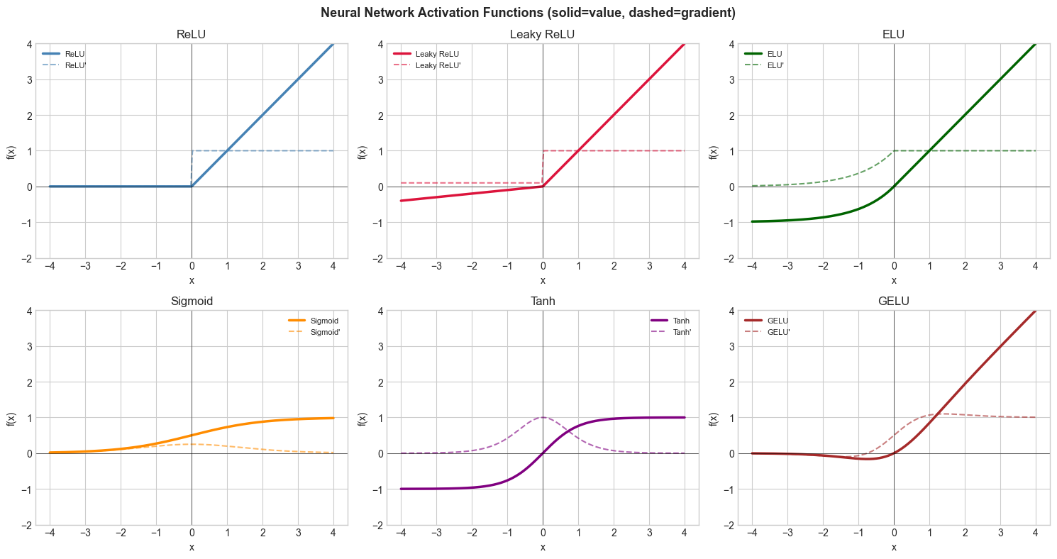
5. Python Implementation
# --- Implementation: Activation benchmarking ---
import numpy as np
import time

ACTIVATIONS = {
    'relu':       lambda x: np.maximum(0, x),
    'sigmoid':    lambda x: 1 / (1 + np.exp(-np.clip(x, -500, 500))),
    'tanh':       np.tanh,
    'leaky_relu': lambda x: np.where(x >= 0, x, 0.1 * x),
    'elu':        lambda x: np.where(x >= 0, x, np.exp(np.minimum(x, 0)) - 1),
    'gelu':       lambda x: x * (1 / (1 + np.exp(-1.702 * x))),
}

def activation_gradient(fn, x, eps=1e-5):
    """Numerical gradient of activation function."""
    return (fn(x + eps) - fn(x - eps)) / (2 * eps)

# Benchmark speed
np.random.seed(0)
x_bench = np.random.randn(1000000)

print("Activation benchmarks (1M elements):")
for name, fn in ACTIVATIONS.items():
    t0 = time.time()
    _ = fn(x_bench)
    elapsed = (time.time() - t0) * 1000
    print(f"  {name:12s}: {elapsed:.2f} ms")

# Gradient check at x=1
print("\nGradient at x=1:")
for name, fn in ACTIVATIONS.items():
    g = activation_gradient(fn, np.array([1.0]))[0]
    print(f"  {name:12s}: {g:.4f}")
Activation benchmarks (1M elements):
relu : 5.81 ms
sigmoid : 45.32 ms
tanh : 23.83 ms
leaky_relu : 15.14 ms
elu : 39.00 ms
gelu : 39.73 ms
Gradient at x=1:
relu : 1.0000
sigmoid : 0.1966
tanh : 0.4200
leaky_relu : 1.0000
elu : 1.0000
gelu : 1.0678
6. Experiments
Experiment 1: Build a 2-layer network manually: output = sigmoid(W2 @ relu(W1 @ x + b1) + b2). Replace relu with sigmoid in layer 1. Does the output change? (Yes — different activation = different learned function space.)
Experiment 2: Check the vanishing gradient problem: compute the gradient of sigmoid(sigmoid(sigmoid(x))) at x=0, x=2, x=5. Watch how the gradient magnitude drops with each sigmoid layer.
7. Exercises
Easy 1. Compute ReLU(-3), ReLU(0), ReLU(0.5). Write ReLU using only max (no if). (Expected: 0, 0, 0.5)
Easy 2. The Leaky ReLU with α=0 becomes standard ReLU. With α=1 it becomes the identity. Verify both cases.
Medium 1. Implement SELU: f(x) = λ(x if x>0, else α(e^x - 1)), where λ≈1.0507, α≈1.6733. These constants are chosen so that the function is self-normalizing. Test that mean and variance of SELU outputs are near 0 and 1 for standard normal input.
Medium 2. Plot the ‘gradient landscape’ of a 3-layer sigmoid network vs 3-layer ReLU network: for 1000 random inputs, compute the numerical gradient. Which maintains larger gradients deeper in the network?
Hard. Implement the Maxout activation: max(w₁ᵀx + b₁, w₂ᵀx + b₂). Show that ReLU is a special case of Maxout. Implement and verify on a simple 1D example.
9. Chapter Summary & Connections
Nonlinear activations enable universal approximation — without them, deep networks = shallow linear transform
Sigmoid/tanh saturate: gradients vanish for large |x|; ReLU doesn’t saturate for x>0
Dying ReLU problem: neurons with only negative inputs produce zero gradient forever
GELU, Swish: smooth variants used in transformers and modern architectures
Backward connection: This unifies ch062–064 into a catalog of tools for ML practitioners.
Forward connections:
ch215 (Chain Rule) explains why vanishing gradients are mathematically inevitable with saturating activations
ch216 (Backpropagation) computes activation gradients layer by layer
The full network is revisited in ch178 (Neural Network Layer Implementation)